Unsupervised Learning of Finite Mixture Models Mrio A

Unsupervised Learning of Finite Mixture Models Mário A. T. Figueiredo mtf@lx. it. pt http: //red. lx. it. pt/~mtf Institute of Telecommunications, and Instituto Superior Técnico. Technical University of Lisbon PORTUGAL This work was done jointly with Anil K. Jain, Michigan State University

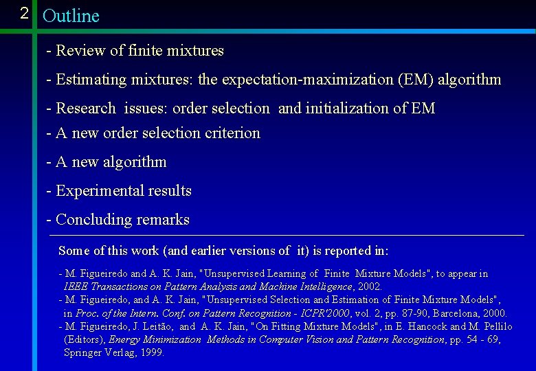
2 Outline - Review of finite mixtures - Estimating mixtures: the expectation-maximization (EM) algorithm - Research issues: order selection and initialization of EM - A new order selection criterion - A new algorithm - Experimental results - Concluding remarks Some of this work (and earlier versions of it) is reported in: - M. Figueiredo and A. K. Jain, "Unsupervised Learning of Finite Mixture Models", to appear in IEEE Transactions on Pattern Analysis and Machine Intelligence, 2002. - M. Figueiredo, and A. K. Jain, "Unsupervised Selection and Estimation of Finite Mixture Models", in Proc. of the Intern. Conf. on Pattern Recognition - ICPR'2000, vol. 2, pp. 87 -90, Barcelona, 2000. - M. Figueiredo, J. Leitão, and A. K. Jain, "On Fitting Mixture Models", in E. Hancock and M. Pellilo (Editors), Energy Minimization Methods in Computer Vision and Pattern Recognition, pp. 54 - 69, Springer Verlag, 1999.

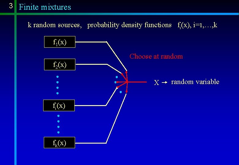
3 Finite mixtures k random sources, probability density functions fi(x), i=1, …, k f 1(x) Choose at random f 2(x) X fi(x) fk(x) random variable

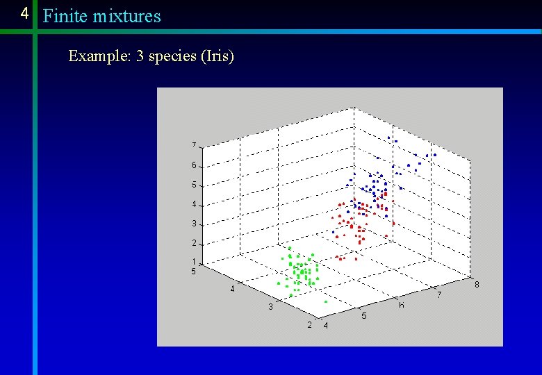
4 Finite mixtures Example: 3 species (Iris)

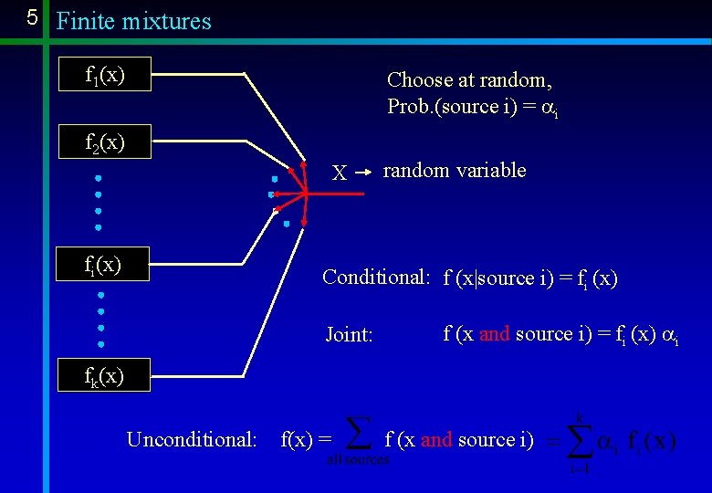
5 Finite mixtures f 1(x) Choose at random, Prob. (source i) = ai f 2(x) X fi(x) random variable Conditional: f (x|source i) = fi (x) Joint: f (x and source i) = fi (x) ai fk(x) Unconditional: f(x) = f (x and source i)

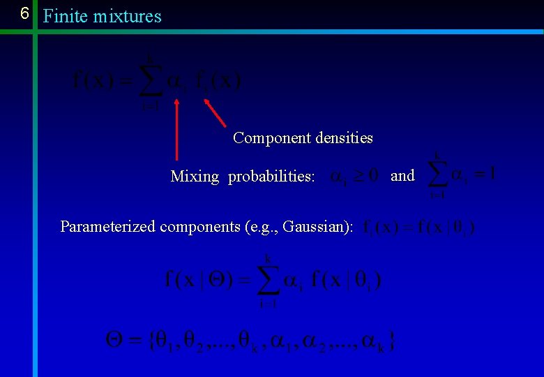
6 Finite mixtures Component densities Mixing probabilities: Parameterized components (e. g. , Gaussian): and

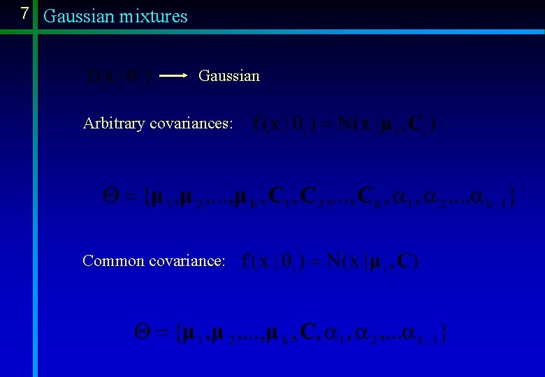
7 Gaussian mixtures Gaussian Arbitrary covariances: Common covariance:

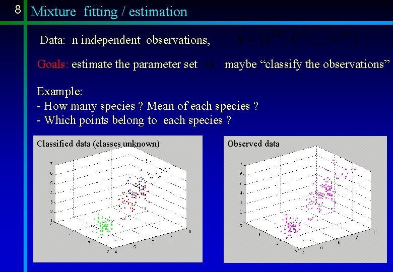
8 Mixture fitting / estimation Data: n independent observations, Goals: estimate the parameter set maybe “classify the observations” Example: - How many species ? Mean of each species ? - Which points belong to each species ? Classified data (classes unknown) Observed data

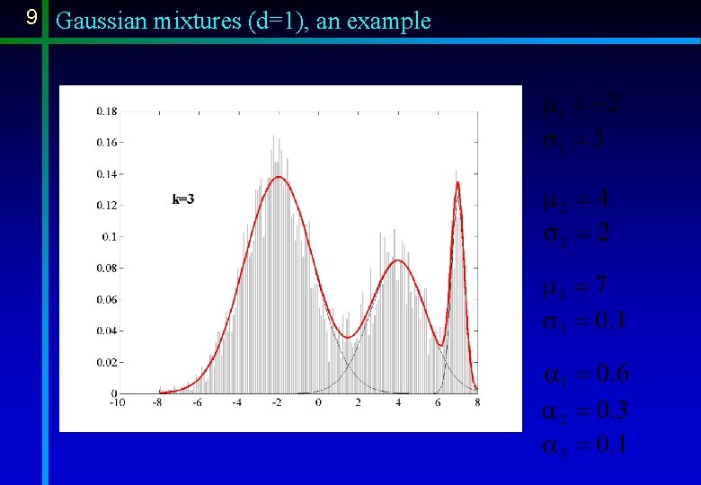
9 Gaussian mixtures (d=1), an example

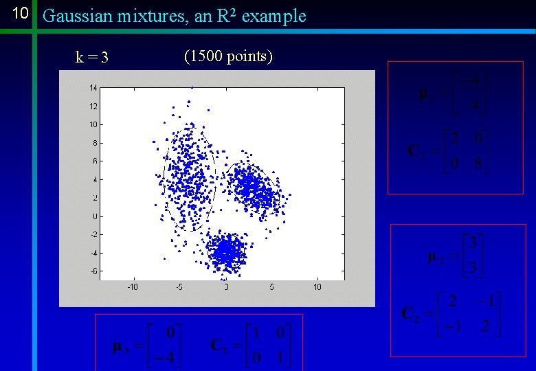
10 Gaussian mixtures, an R 2 example k=3 (1500 points)

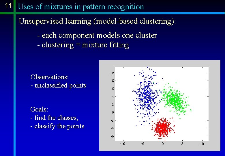
11 Uses of mixtures in pattern recognition Unsupervised learning (model-based clustering): - each component models one cluster - clustering = mixture fitting Observations: - unclassified points Goals: - find the classes, - classify the points

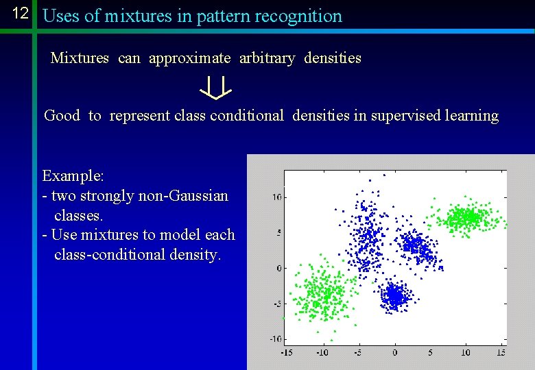
12 Uses of mixtures in pattern recognition Mixtures can approximate arbitrary densities Good to represent class conditional densities in supervised learning Example: - two strongly non-Gaussian classes. - Use mixtures to model each class-conditional density.

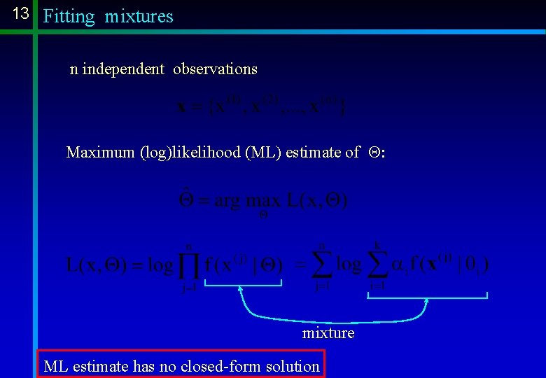
13 Fitting mixtures n independent observations Maximum (log)likelihood (ML) estimate of Q: mixture ML estimate has no closed-form solution

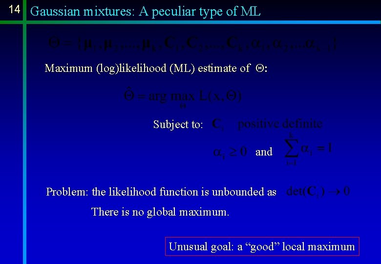
14 Gaussian mixtures: A peculiar type of ML Maximum (log)likelihood (ML) estimate of Q: Subject to: and Problem: the likelihood function is unbounded as There is no global maximum. Unusual goal: a “good” local maximum

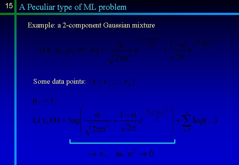
15 A Peculiar type of ML problem Example: a 2 -component Gaussian mixture Some data points:

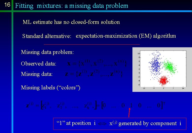
16 Fitting mixtures: a missing data problem ML estimate has no closed-form solution Standard alternative: expectation-maximization (EM) algorithm Missing data problem: Observed data: Missing labels (“colors”) “ 1” at position i x( j) generated by component i

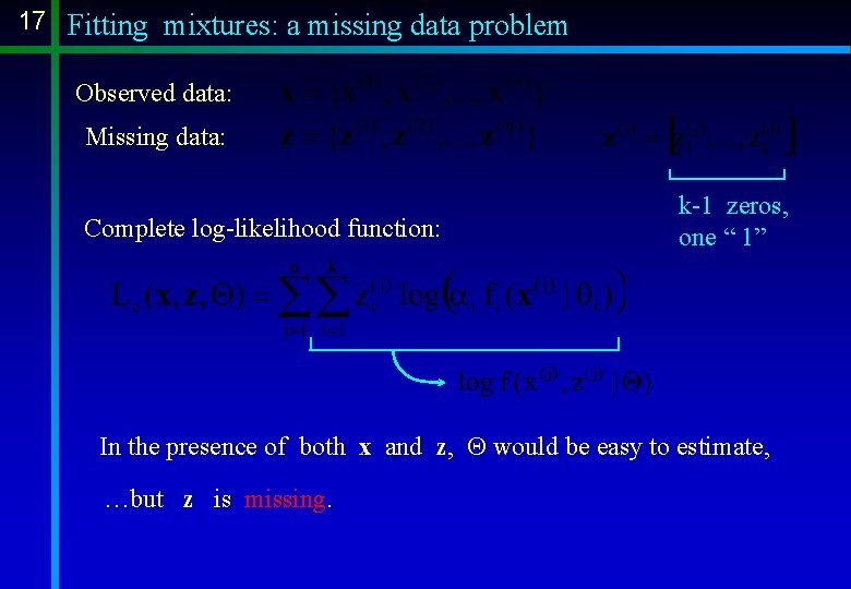
17 Fitting mixtures: a missing data problem Observed data: Missing data: Complete log-likelihood function: k-1 zeros, one “ 1” In the presence of both x and z, Q would be easy to estimate, …but z is missing.

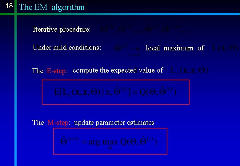
18 The EM algorithm Iterative procedure: Under mild conditions: local maximum of The E-step: compute the expected value of The M-step: update parameter estimates

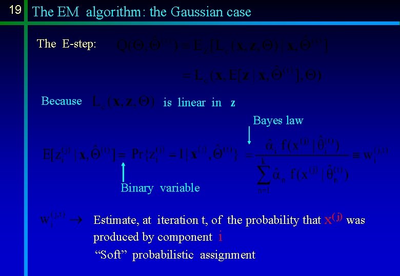
19 The EM algorithm: the Gaussian case The E-step: Because is linear in z Bayes law Binary variable Estimate, at iteration t, of the probability that x( j) was produced by component i “Soft” probabilistic assignment

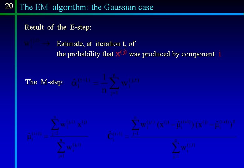
20 The EM algorithm: the Gaussian case Result of the E-step: Estimate, at iteration t, of the probability that x( j) was produced by component i The M-step:

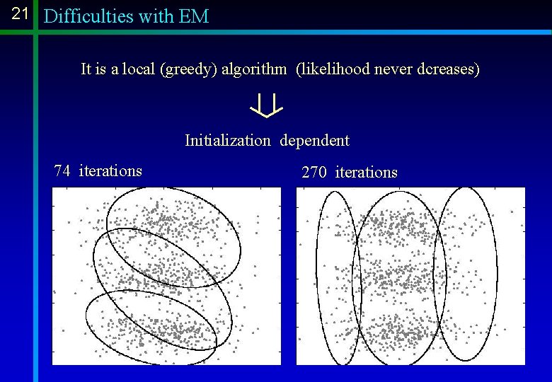
21 Difficulties with EM It is a local (greedy) algorithm (likelihood never dcreases) Initialization dependent 74 iterations 270 iterations

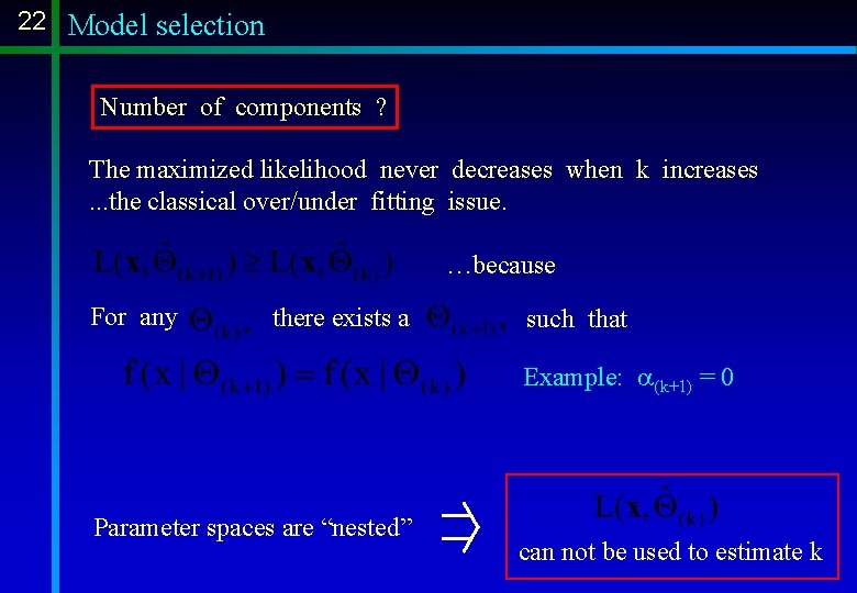
22 Model selection Number of components ? The maximized likelihood never decreases when k increases. . . the classical over/under fitting issue. …because For any there exists a such that Example: a(k+1) = 0 Parameter spaces are “nested” can not be used to estimate k

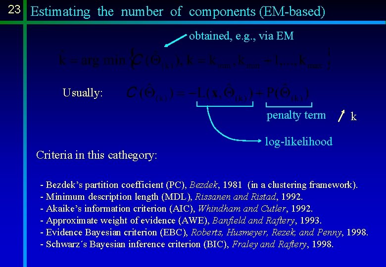
23 Estimating the number of components (EM-based) obtained, e. g. , via EM Usually: penalty term k log-likelihood Criteria in this cathegory: - Bezdek’s partition coefficient (PC), Bezdek, 1981 (in a clustering framework). - Minimum description length (MDL), Rissanen and Ristad, 1992. - Akaike’s information criterion (AIC), Whindham and Cutler, 1992. - Approximate weight of evidence (AWE), Banfield and Raftery, 1993. - Evidence Bayesian criterion (EBC), Roberts, Husmeyer, Rezek, and Penny, 1998. - Schwarz´s Bayesian inference criterion (BIC), Fraley and Raftery, 1998.

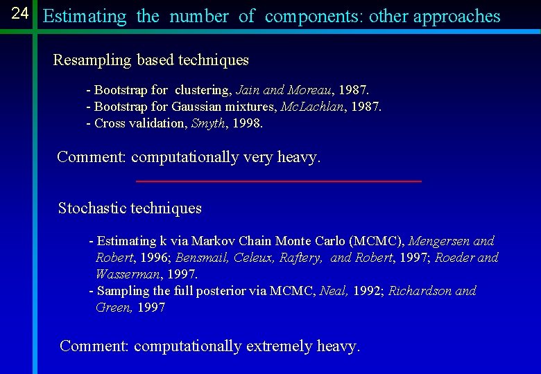
24 Estimating the number of components: other approaches Resampling based techniques - Bootstrap for clustering, Jain and Moreau, 1987. - Bootstrap for Gaussian mixtures, Mc. Lachlan, 1987. - Cross validation, Smyth, 1998. Comment: computationally very heavy. Stochastic techniques - Estimating k via Markov Chain Monte Carlo (MCMC), Mengersen and Robert, 1996; Bensmail, Celeux, Raftery, and Robert, 1997; Roeder and Wasserman, 1997. - Sampling the full posterior via MCMC, Neal, 1992; Richardson and Green, 1997 Comment: computationally extremely heavy.

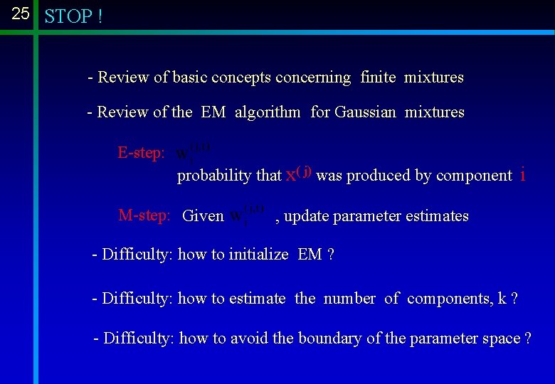
25 STOP ! - Review of basic concepts concerning finite mixtures - Review of the EM algorithm for Gaussian mixtures E-step: probability that x( j) was produced by component i M-step: Given , update parameter estimates - Difficulty: how to initialize EM ? - Difficulty: how to estimate the number of components, k ? - Difficulty: how to avoid the boundary of the parameter space ?

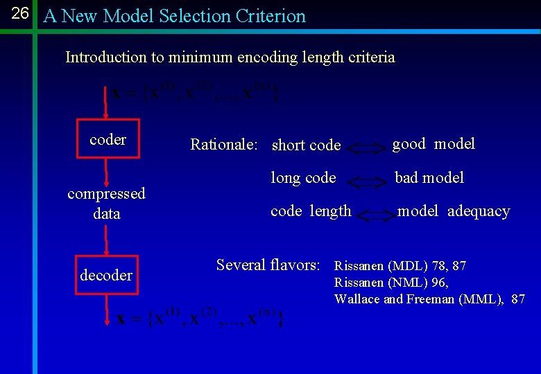
26 A New Model Selection Criterion Introduction to minimum encoding length criteria coder compressed data decoder Rationale: short code good model long code bad model code length model adequacy Several flavors: Rissanen (MDL) 78, 87 Rissanen (NML) 96, Wallace and Freeman (MML), 87

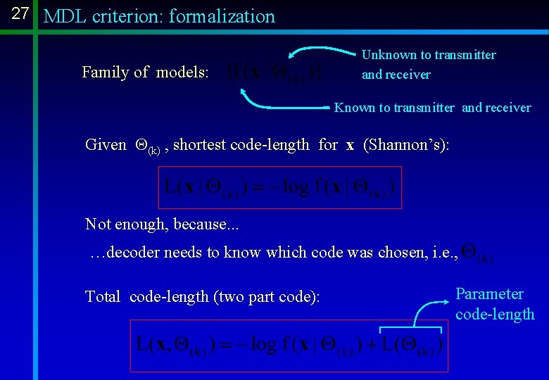
27 MDL criterion: formalization Family of models: Unknown to transmitter and receiver Known to transmitter and receiver Given Q(k) , shortest code-length for x (Shannon’s): Not enough, because. . . …decoder needs to know which code was chosen, i. e. , Total code-length (two part code): Parameter code-length

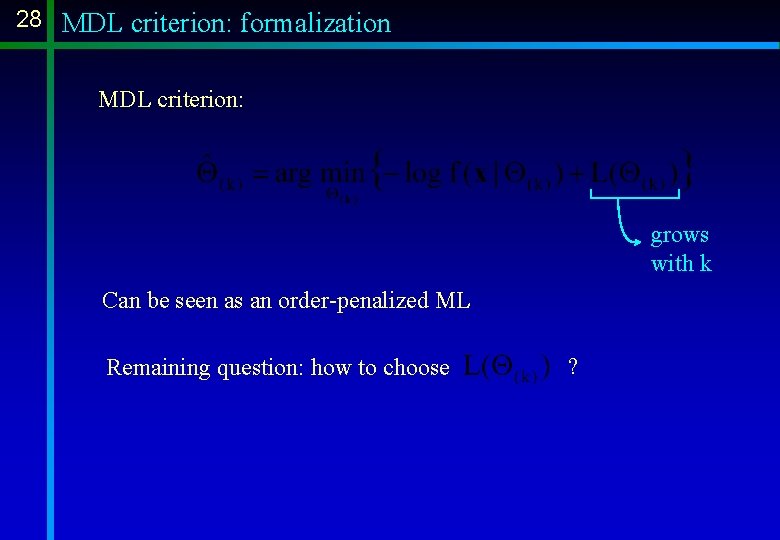
28 MDL criterion: formalization MDL criterion: grows with k Can be seen as an order-penalized ML Remaining question: how to choose ?

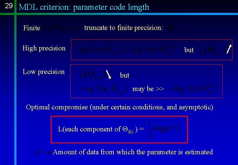
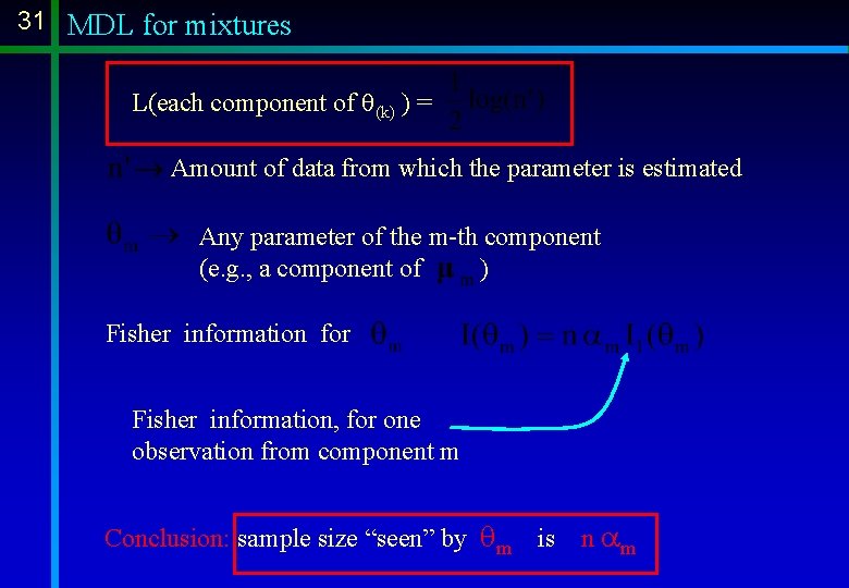
29 MDL criterion: parameter code length truncate to finite precision: Finite High precision Low precision but may be >> Optimal compromise (under certain conditions, and asymptotic) L(each component of Q(k) ) = Amount of data from which the parameter is estimated

30 MDL criterion: parameter code length L[each component of q(k) ] = Amount of data from which the parameter is estimated Classical MDL: n’ = n Not true for mixtures ! Why ? Not all data points have equal weight in each parameter estimate

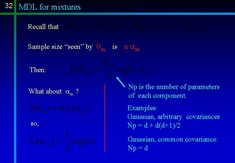
31 MDL for mixtures L(each component of q(k) ) = Amount of data from which the parameter is estimated Any parameter of the m-th component (e. g. , a component of ) Fisher information for Fisher information, for one observation from component m Conclusion: sample size “seen” by qm is n am

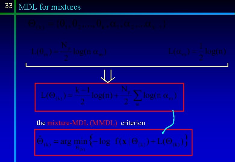
32 MDL for mixtures Recall that Sample size “seen” by qm is n am Then: What about am ? so, Np is the number of parameters of each component. Examples: Gaussian, arbitrary covariances Np = d + d(d+1)/2 Gaussian, common covariance: Np = d

33 MDL for mixtures the mixture-MDL (MMDL) criterion :

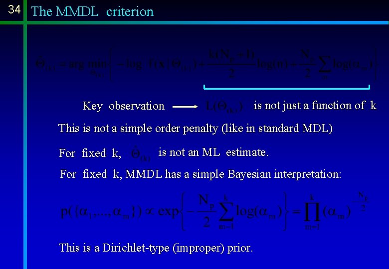
34 The MMDL criterion Key observation is not just a function of k This is not a simple order penalty (like in standard MDL) For fixed k, is not an ML estimate. For fixed k, MMDL has a simple Bayesian interpretation: This is a Dirichlet-type (improper) prior.

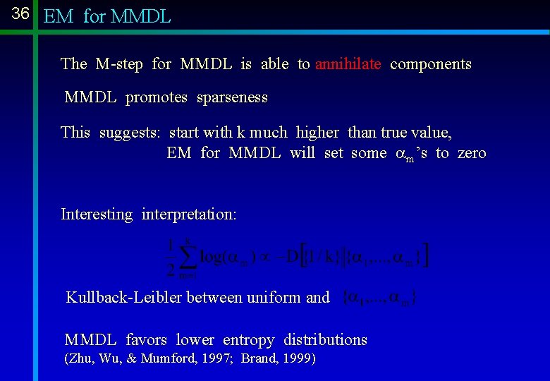
35 EM for MMDL Using EM redefining the M-step (there is a prior on the am’s) Simple, because Dirichlet is conjugate y+ y because of constraints Remarkable fact: this M-step may annihilate components

36 EM for MMDL The M-step for MMDL is able to annihilate components MMDL promotes sparseness This suggests: start with k much higher than true value, EM for MMDL will set some am’s to zero Interesting interpretation: Kullback-Leibler between uniform and MMDL favors lower entropy distributions (Zhu, Wu, & Mumford, 1997; Brand, 1999)

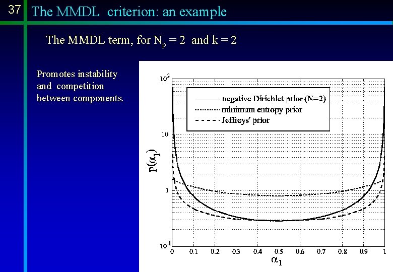
37 The MMDL criterion: an example The MMDL term, for Np = 2 and k = 2 Promotes instability and competition between components.

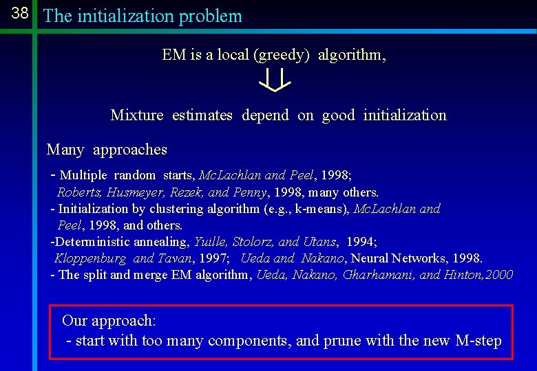
38 The initialization problem EM is a local (greedy) algorithm, Mixture estimates depend on good initialization Many approaches - Multiple random starts, Mc. Lachlan and Peel, 1998; Roberts, Husmeyer, Rezek, and Penny, 1998, many others. - Initialization by clustering algorithm (e. g. , k-means), Mc. Lachlan and Peel, 1998, and others. -Deterministic annealing, Yuille, Stolorz, and Utans, 1994; Kloppenburg and Tavan, 1997; Ueda and Nakano, Neural Networks, 1998. - The split and merge EM algorithm, Ueda, Nakano, Gharhamani, and Hinton, 2000 Our approach: - start with too many components, and prune with the new M-step

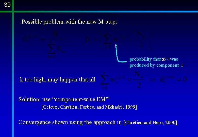
39 Possible problem with the new M-step: probability that x( j) was produced by component i k too high, may happen that all Solution: use “component-wise EM” [Celeux, Chrétien, Forbes, and Mkhadri, 1999] Convergence shown using the approach in [Chrétien and Hero, 2000]

40 Component-wise EM [Celeux, Chrétien, Forbes, and Mkhadri, 1999] - Update - Recompute all the -. . Repeat until convergence - Update - Recompute all the Key fact: if one componend “dies”, its probability mass is immediately re-distributed

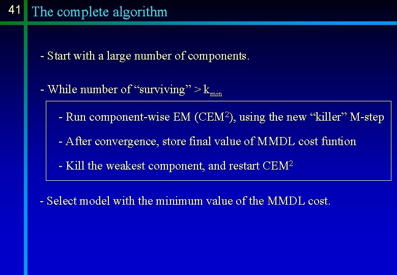
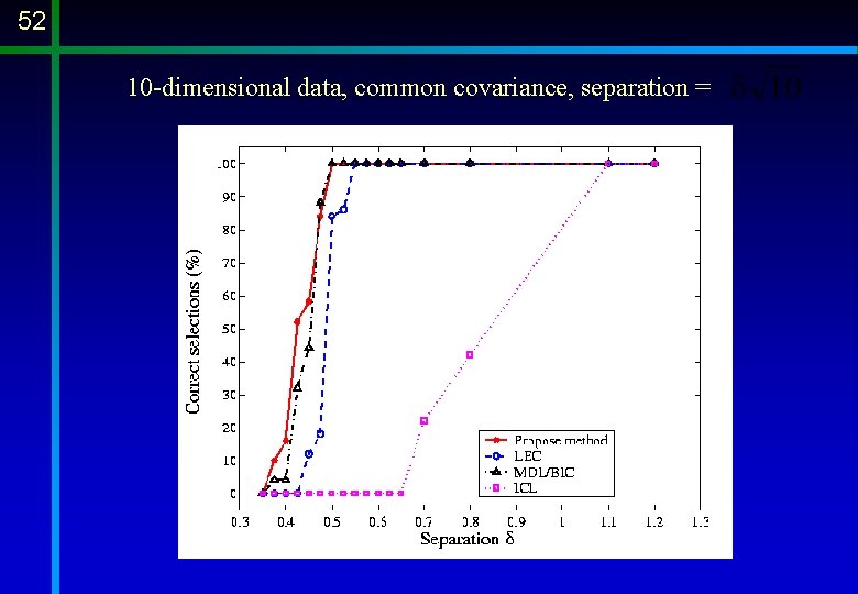
41 The complete algorithm - Start with a large number of components. - While number of “surviving” > kmin - Run component-wise EM (CEM 2), using the new “killer” M-step - After convergence, store final value of MMDL cost funtion - Kill the weakest component, and restart CEM 2 - Select model with the minimum value of the MMDL cost.

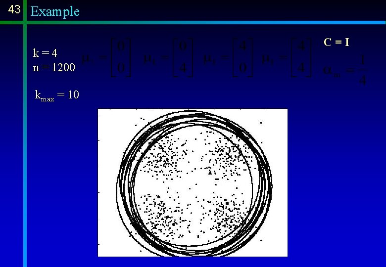
42 Example Same as in [Ueda and Nakano, 1998].

43 Example k=4 n = 1200 kmax = 10 C=I

44 Example Same as in [Ueda, Nakano, Ghahramani and Hinton, 2000].

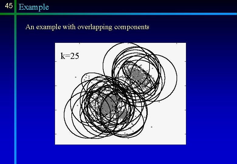
45 Example An example with overlapping components

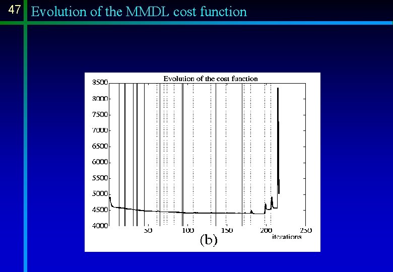
46 Evolution of the MMDL cost function

47 Evolution of the MMDL cost function

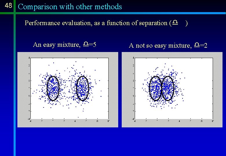
48 Comparison with other methods Performance evaluation, as a function of separation (d An easy mixture, d=5 ) A not so easy mixture, d=2

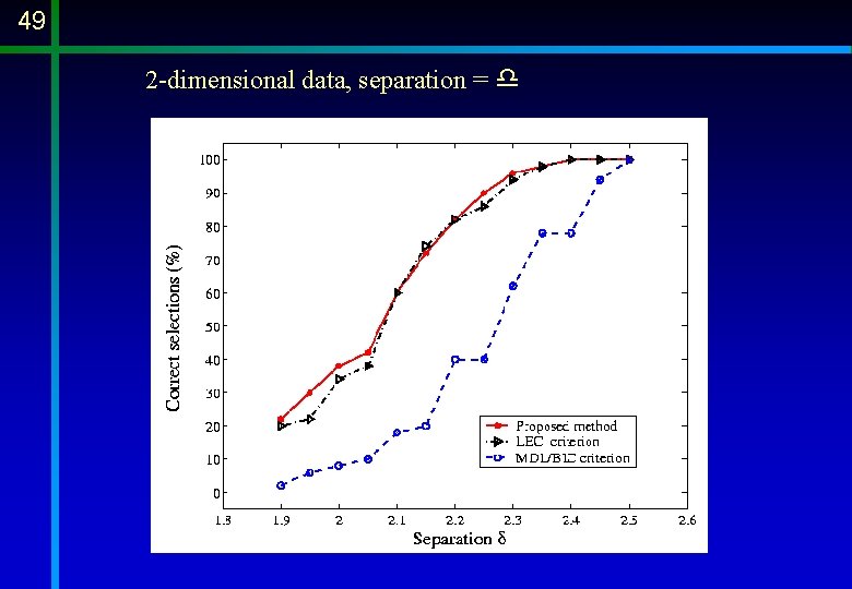
49 2 -dimensional data, separation = d

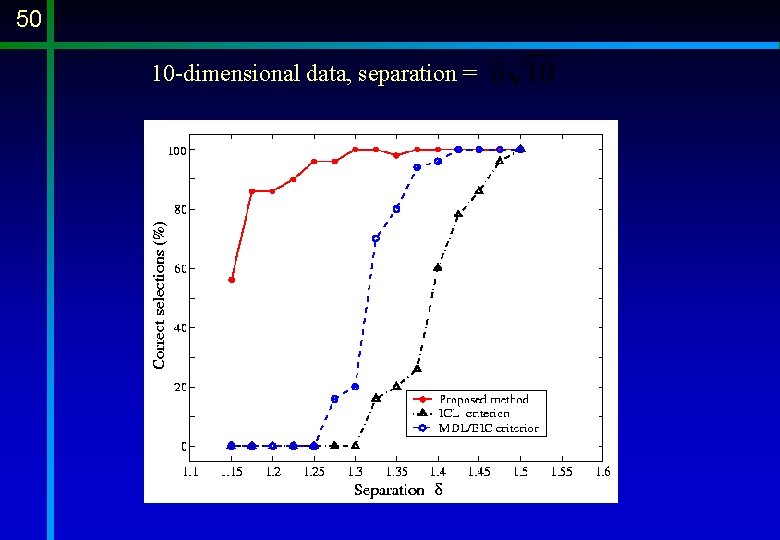
50 10 -dimensional data, separation =

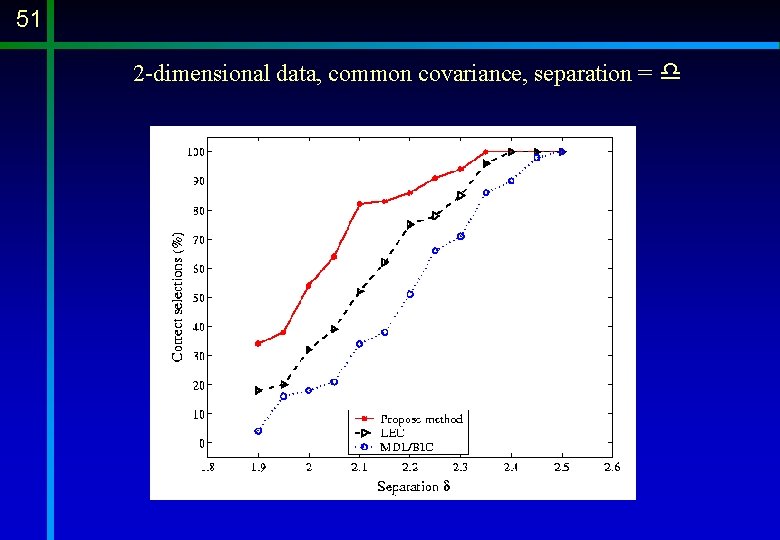
51 2 -dimensional data, common covariance, separation = d

52 10 -dimensional data, common covariance, separation =

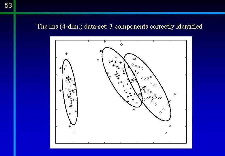
53 The iris (4 -dim. ) data-set: 3 components correctly identified

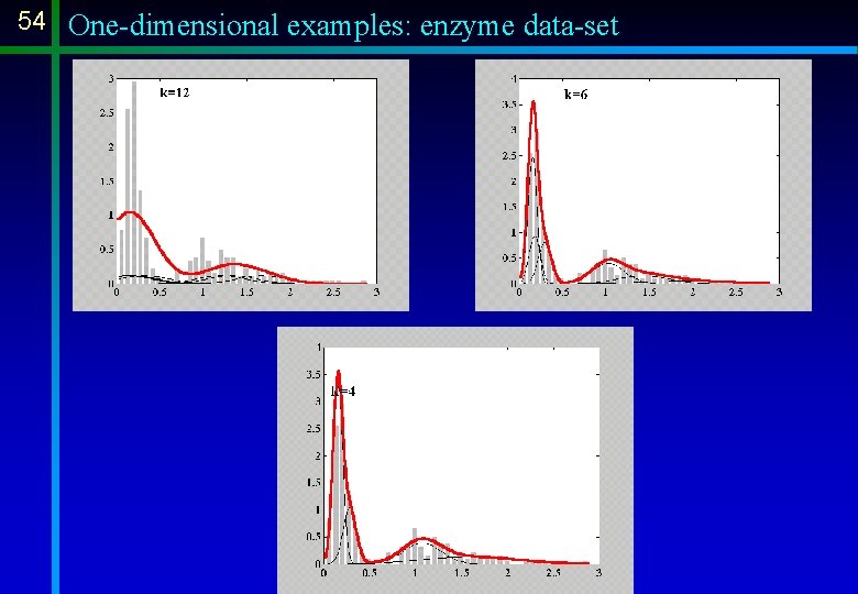
54 One-dimensional examples: enzyme data-set

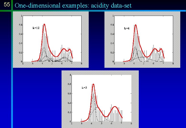
55 One-dimensional examples: acidity data-set

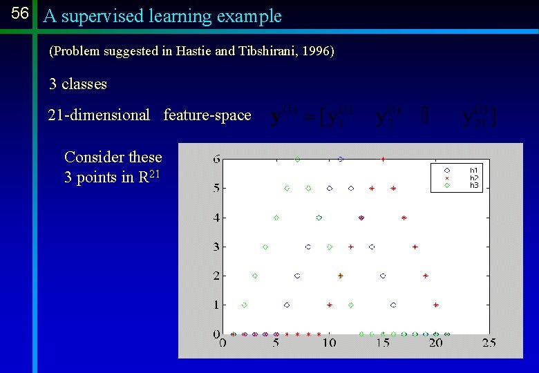
56 A supervised learning example (Problem suggested in Hastie and Tibshirani, 1996) 3 classes 21 -dimensional feature-space Consider these 3 points in R 21

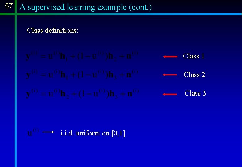
57 A supervised learning example (cont. ) Class definitions: Class 1 Class 2 Class 3 i. i. d. uniform on [0, 1]

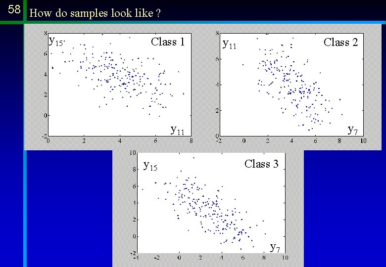
58 How do samples look like ? y 15 Class 1 y 11 Class 2 y 11 y 15 y 7 Class 3 y 7

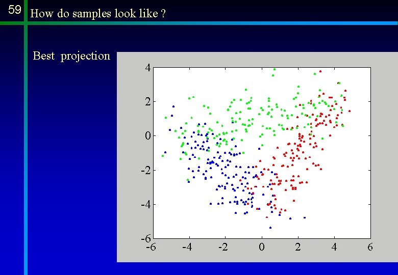
59 How do samples look like ? Best projection

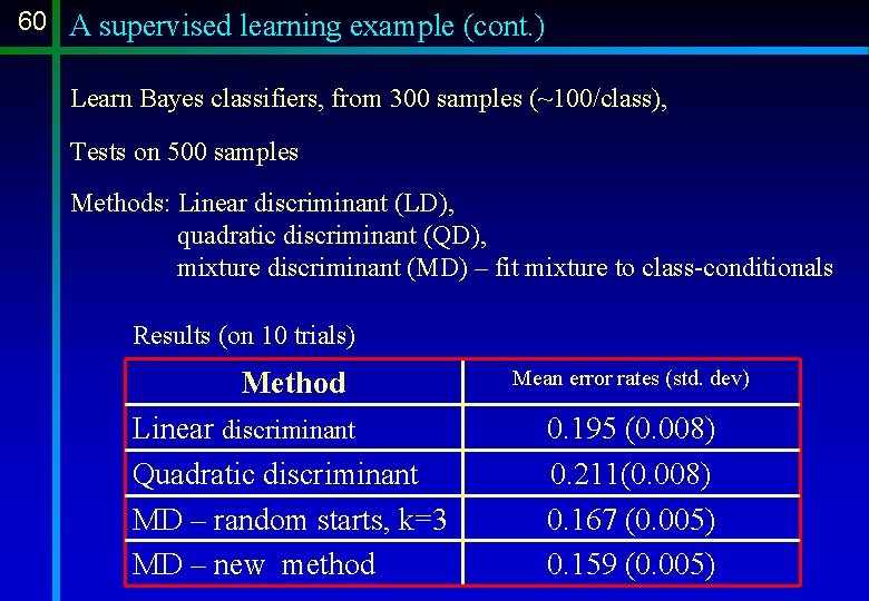
60 A supervised learning example (cont. ) Learn Bayes classifiers, from 300 samples (~100/class), Tests on 500 samples Methods: Linear discriminant (LD), quadratic discriminant (QD), mixture discriminant (MD) – fit mixture to class-conditionals Results (on 10 trials) Method Mean error rates (std. dev) Linear discriminant Quadratic discriminant MD – random starts, k=3 MD – new method 0. 195 (0. 008) 0. 211(0. 008) 0. 167 (0. 005) 0. 159 (0. 005)

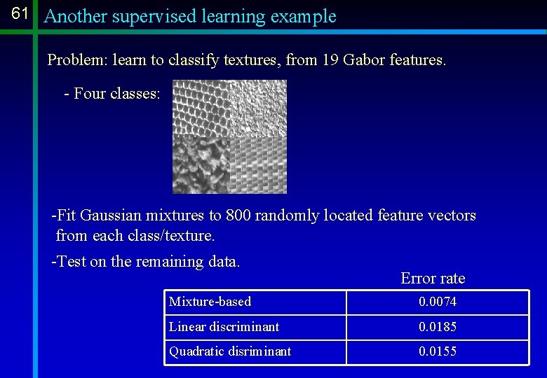
61 Another supervised learning example Problem: learn to classify textures, from 19 Gabor features. - Four classes: -Fit Gaussian mixtures to 800 randomly located feature vectors from each class/texture. -Test on the remaining data. Error rate Mixture-based 0. 0074 Linear discriminant 0. 0185 Quadratic disriminant 0. 0155

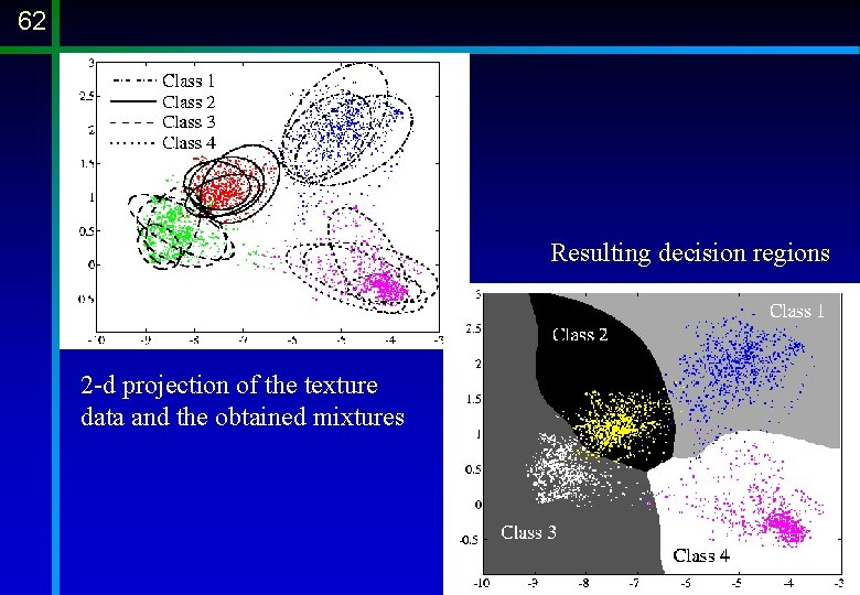
62 Resulting decision regions 2 -d projection of the texture data and the obtained mixtures

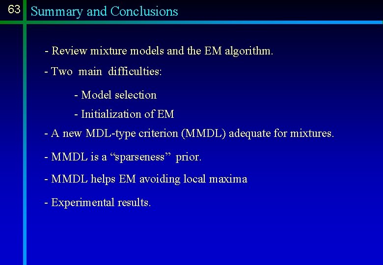
63 Summary and Conclusions - Review mixture models and the EM algorithm. - Two main difficulties: - Model selection - Initialization of EM - A new MDL-type criterion (MMDL) adequate for mixtures. - MMDL is a “sparseness” prior. - MMDL helps EM avoiding local maxima - Experimental results.