Unsupervised Learning by Convex and Conic Coding D

Unsupervised Learning by Convex and Conic Coding D. D. Lee and H. S. Seung NIPS’ 1997

Introduction n Learning algorithms based on convex and conic encoders are introduced. – Less constrained than VQ but more constrained than PCA. » VQ n n n Encode each input as the index of the closest prototype. Capture nonlinear structure Highly localized » PCA n n n Encode as the coefficient of a linear superposition of a set of basis vectors. Distributed representation Can only model linear structures.

– Can produce sparse distributed representation. – Learning algorithms can be understood as approximate matrix factorization.

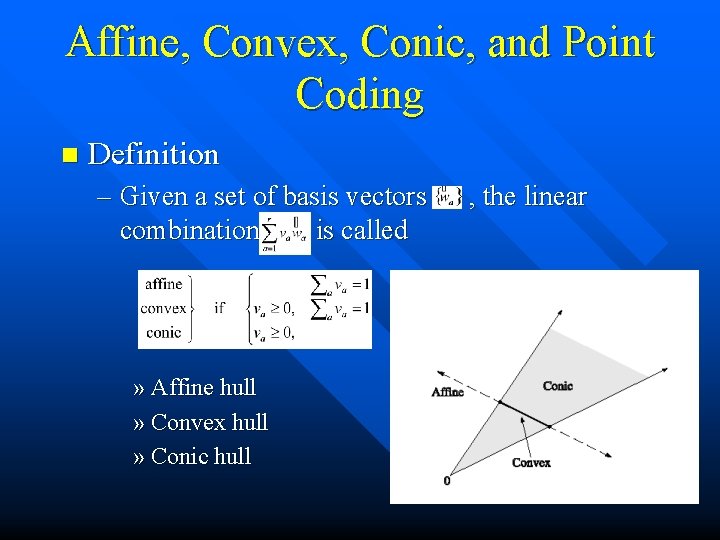
Affine, Convex, Conic, and Point Coding n Definition – Given a set of basis vectors combination is called » Affine hull » Convex hull » Conic hull , the linear

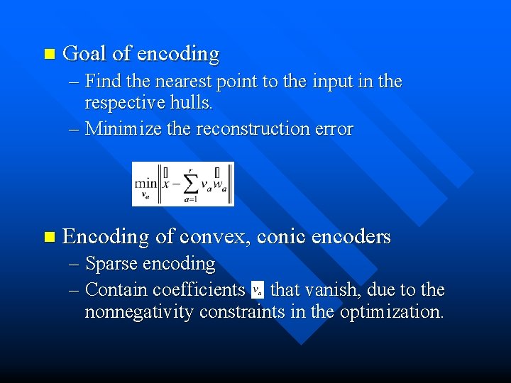
n Goal of encoding – Find the nearest point to the input in the respective hulls. – Minimize the reconstruction error n Encoding of convex, conic encoders – Sparse encoding – Contain coefficients that vanish, due to the nonnegativity constraints in the optimization.

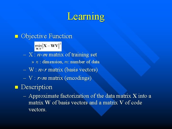
Learning n Objective Function – X : n m matrix of training set » n : dimension, m: number of data – W : n r matrix (basis vectors) – V : r m matrix (encodings) n Description – Approximate factorization of the data matrix X into a matrix W of basis vectors and a matrix V of code vectors.

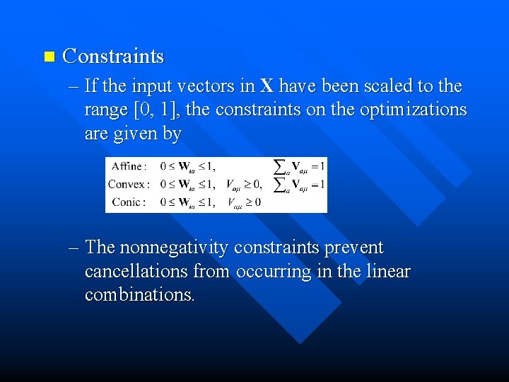
n Constraints – If the input vectors in X have been scaled to the range [0, 1], the constraints on the optimizations are given by – The nonnegativity constraints prevent cancellations from occurring in the linear combinations.

Example: modeling handwritten digits n Experimental Setup – Affine, Convex, Conic, and VQ learning to the USPS database. » Handwritten digits segmented from actual zip codes. » 7291 training and 2007 test images were normalized to a 16 16 grid with pixel intensities in the range [0, 1]. – Training examples were segregated by digit class. – Separate basis vectors were trained for each of the classes using four encodings.

n VQ – k-means algorithm was used – Restarted with various initial conditions and the best solution was chosen. n Affine – Determine the affine space that best models the input data. – No obvious interpretation. n Convex – Finds the r basis vectors whose convex hull best fits the input data. – Alternate between projected gradient steps of W and V. – The basis vectors are interpretable as templates and are less blurred than those found in VQ. – Eliminate many invariant transformations, because they would violate the nonnegativity constraints.

n Conic – Finds basis vectors whose conic hull best models the input images. – Representation allows combinations of basis vectors. – The basis vectors found are features rather than templates.

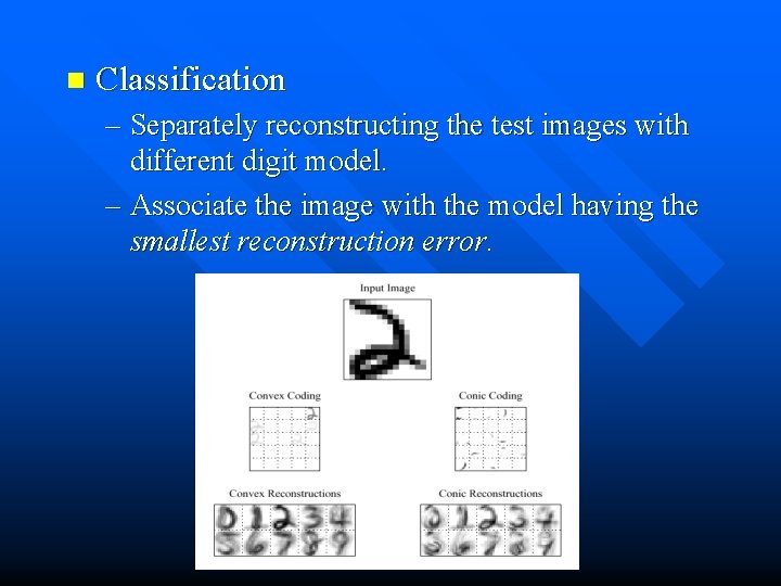
n Classification – Separately reconstructing the test images with different digit model. – Associate the image with the model having the smallest reconstruction error.

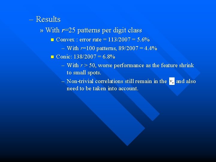
– Results » With r=25 patterns per digit class Convex : error rate = 113/2007 = 5. 6% – With r=100 patterns, 89/2007 = 4. 4% n Conic: 138/2007 = 6. 8% – With r > 50, worse performance as the feature shrink to small spots. – Non-trivial correlations still remain in the and also need to be taken into account. n

Discussion n n Convex coding is similar to other locally linear models. Conic coding is similar to the noisy OR and harmonium models – Conic uses continuous variables rather than binary variables. » Makes the encoding computationally tractable and allows for interpolation between basis vectors. n Convex and Conic coding is can be viewed as probabilistic latent variable models. – No explicit model P(va) for the hidden variables was used. » Limit the quality of the Conic models n Building hierarchical representations is needed.