University of Washington EMBA Program Regional 20 Conjoint

University of Washington EMBA Program Regional 20 “Conjoint Analysis” TA: Rory Mc. Leod October 7, 2003

What is Conjoint Analysis? • A quantitative analysis used to estimate customers’ value systems • Requires that a product be broken down into a set of attributes • Value system: how much value a consumer puts on each level of each of the attributes

Uses of Conjoint Analysis • Learning more about your potential customer segments – Further market segmentation • New product development – Extending types of products within a category – Entering a new category • Determining optimal positioning

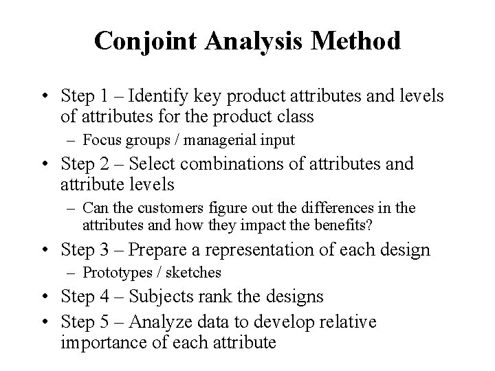
Conjoint Analysis Method • Step 1 – Identify key product attributes and levels of attributes for the product class – Focus groups / managerial input • Step 2 – Select combinations of attributes and attribute levels – Can the customers figure out the differences in the attributes and how they impact the benefits? • Step 3 – Prepare a representation of each design – Prototypes / sketches • Step 4 – Subjects rank the designs • Step 5 – Analyze data to develop relative importance of each attribute

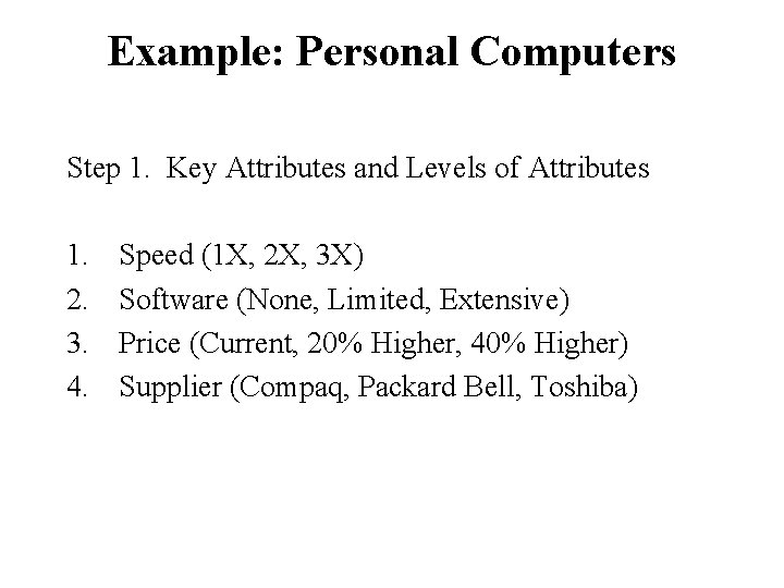
Example: Personal Computers Step 1. Key Attributes and Levels of Attributes 1. 2. 3. 4. Speed (1 X, 2 X, 3 X) Software (None, Limited, Extensive) Price (Current, 20% Higher, 40% Higher) Supplier (Compaq, Packard Bell, Toshiba)

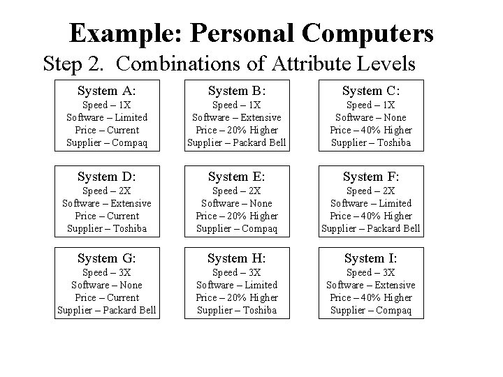
Example: Personal Computers Step 2. Combinations of Attribute Levels System A: System B: System C: Speed – 1 X Software – Limited Price – Current Supplier – Compaq Speed – 1 X Software – Extensive Price – 20% Higher Supplier – Packard Bell Speed – 1 X Software – None Price – 40% Higher Supplier – Toshiba System D: System E: System F: Speed – 2 X Software – Extensive Price – Current Supplier – Toshiba Speed – 2 X Software – None Price – 20% Higher Supplier – Compaq Speed – 2 X Software – Limited Price – 40% Higher Supplier – Packard Bell System G: System H: System I: Speed – 3 X Software – None Price – Current Supplier – Packard Bell Speed – 3 X Software – Limited Price – 20% Higher Supplier – Toshiba Speed – 3 X Software – Extensive Price – 40% Higher Supplier – Compaq Use software to select product combinations such that attributes are uncorrelated (orthogonal).

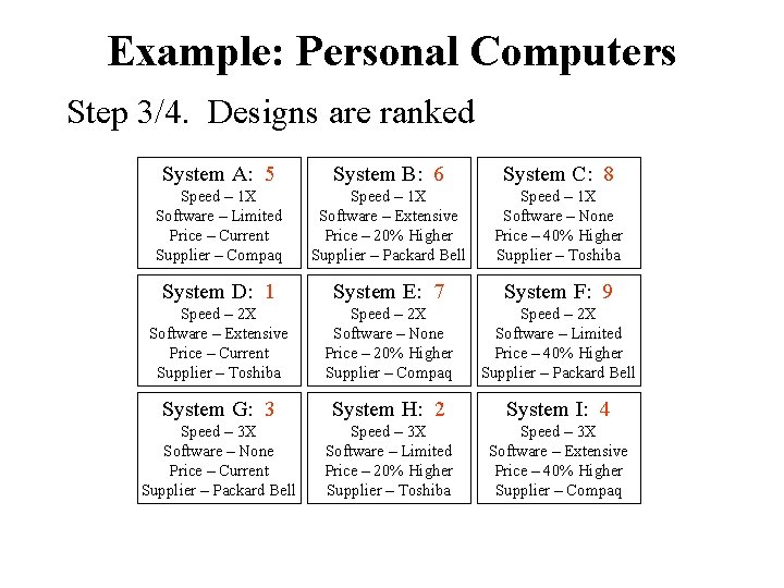
Example: Personal Computers Step 3/4. Designs are ranked System A: 5 System B: 6 System C: 8 Speed – 1 X Software – Limited Price – Current Supplier – Compaq Speed – 1 X Software – Extensive Price – 20% Higher Supplier – Packard Bell Speed – 1 X Software – None Price – 40% Higher Supplier – Toshiba System D: 1 System E: 7 System F: 9 Speed – 2 X Software – Extensive Price – Current Supplier – Toshiba Speed – 2 X Software – None Price – 20% Higher Supplier – Compaq Speed – 2 X Software – Limited Price – 40% Higher Supplier – Packard Bell System G: 3 System H: 2 System I: 4 Speed – 3 X Software – None Price – Current Supplier – Packard Bell Speed – 3 X Software – Limited Price – 20% Higher Supplier – Toshiba Speed – 3 X Software – Extensive Price – 40% Higher Supplier – Compaq Customer Preference (most preferred to least): D, H, G, I, A, B, E, C, F

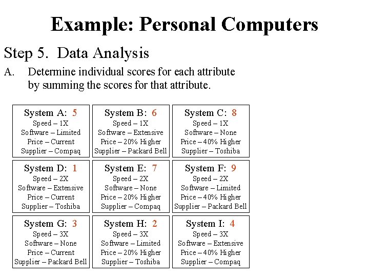
Example: Personal Computers Step 5. Data Analysis A. Determine individual scores for each attribute by summing the scores for that attribute. System A: 5 System B: 6 System C: 8 Speed – 1 X Software – Limited Price – Current Supplier – Compaq Speed – 1 X Software – Extensive Price – 20% Higher Supplier – Packard Bell Speed – 1 X Software – None Price – 40% Higher Supplier – Toshiba System D: 1 System E: 7 System F: 9 Speed – 2 X Software – Extensive Price – Current Supplier – Toshiba Speed – 2 X Software – None Price – 20% Higher Supplier – Compaq Speed – 2 X Software – Limited Price – 40% Higher Supplier – Packard Bell System G: 3 System H: 2 System I: 4 Speed – 3 X Software – None Price – Current Supplier – Packard Bell Speed – 3 X Software – Limited Price – 20% Higher Supplier – Toshiba Speed – 3 X Software – Extensive Price – 40% Higher Supplier – Compaq Software: None = 8+7+3 = 18 Limited = 5+9+2 = 16 Extensive = 6+1+4 = 11 Manufacturer: Compaq = 5+7+4 = 16 Toshiba = 8+1+2 = 11 Packard Bell = 6+1+4 = 11 Price: Current = 5+1+3 = 9 20% Higher = 6+7+2 = 15 40% Higher = 8+9+4 = 21 Speed: 1 X = 5+6+8 = 19 2 X = 1+7+9 = 17 3 X = 3+2+4 = 9

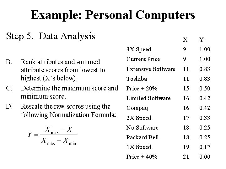
Example: Personal Computers Step 5. Data Analysis B. C. D. Rank attributes and summed attribute scores from lowest to highest (X’s below). Determine the maximum score and minimum score. Rescale the raw scores using the following Normalization Formula: X Y 3 X Speed 9 1. 00 Current Price 9 1. 00 Extensive Software 11 0. 83 Toshiba 11 0. 83 Price + 20% 15 0. 50 Limited Software 16 0. 42 Compaq 16 0. 42 2 X Speed 17 0. 33 No Software 18 0. 25 Packard Bell 18 0. 25 1 X Speed 19 0. 17 Price + 40% 21 0. 00

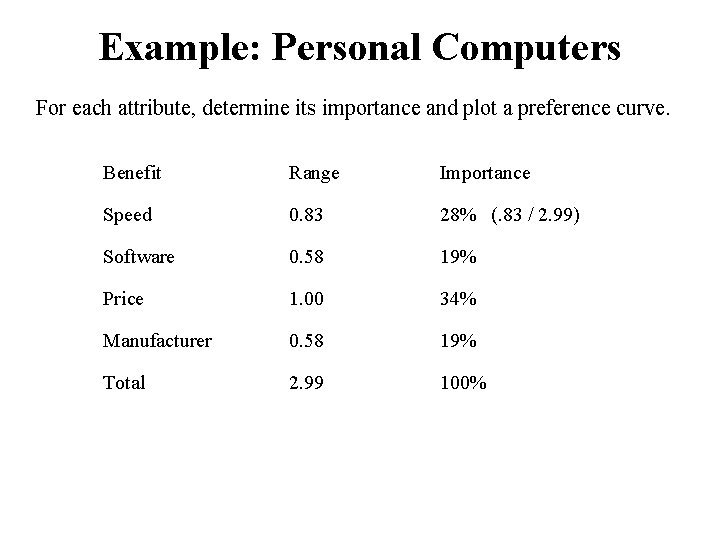
Example: Personal Computers For each attribute, determine its importance and plot a preference curve. Benefit Range Importance Speed 0. 83 28% (. 83 / 2. 99) Software 0. 58 19% Price 1. 00 34% Manufacturer 0. 58 19% Total 2. 99 100%

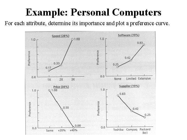
Example: Personal Computers For each attribute, determine its importance and plot a preference curve.

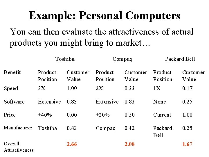
Example: Personal Computers You can then evaluate the attractiveness of actual products you might bring to market… Toshiba Compaq Packard Bell Benefit Product Position Customer Value Speed 3 X 1. 00 2 X 0. 33 1 X 0. 17 Software Extensive 0. 83 None 0. 25 Price +40% 0. 00 +20% 0. 50 Current 1. 00 Manufacturer Toshiba 0. 83 Compaq 0. 42 Packard Bell 0. 25 Overall Attractiveness 2. 66 2. 08 1. 67

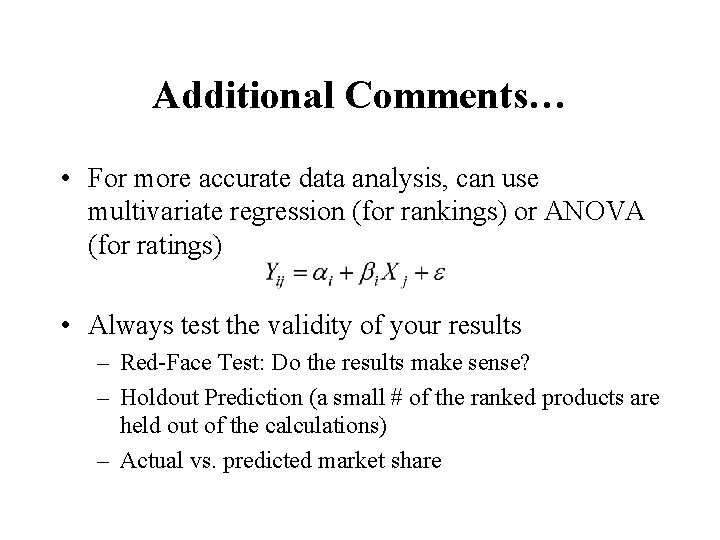
Additional Comments… • For more accurate data analysis, can use multivariate regression (for rankings) or ANOVA (for ratings) • Always test the validity of your results – Red-Face Test: Do the results make sense? – Holdout Prediction (a small # of the ranked products are held out of the calculations) – Actual vs. predicted market share