University of British Columbia CPSC 414 Computer Graphics

University of British Columbia CPSC 414 Computer Graphics Scan Conversion Week 6, Wed 8 Oct 2003 • recap: polygon scan conversion • interpolation • barycentric coords • transforming normals • sampling © Tamara Munzner 1

• Homework 1 News – problem 18 • x and y transposed in bottom layer – problem 4 • rotate 30 deg around x axis with fixed point of (3, 5, 12, 1) – new correct PDF posted – reminder: no late work after Fri 17 Oct 9 am • handin box 18 CICSR basement • Project 1 – solution, hall of fame on Friday Week 6, Wed 8 Oct 03 © Tamara Munzner 2

News • Office hours reminder: FSC 2618 – Mondays 10: 30 -11: 30 or by appointment – exceptions: Oct 20, Nov 10 • Readings – Chap 8. 9 -8. 11, Fri 10/3 slide notes Week 6, Wed 8 Oct 03 © Tamara Munzner 3

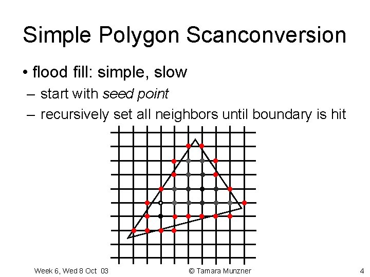
Simple Polygon Scanconversion • flood fill: simple, slow – start with seed point – recursively set all neighbors until boundary is hit Week 6, Wed 8 Oct 03 © Tamara Munzner 4

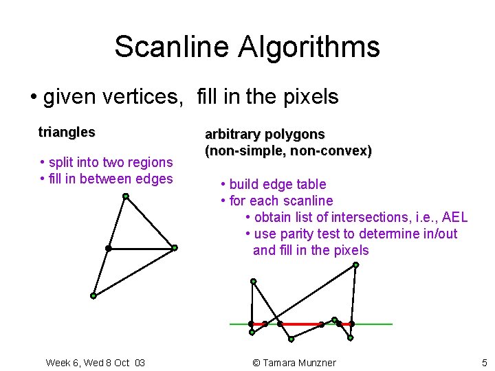
Scanline Algorithms • given vertices, fill in the pixels triangles • split into two regions • fill in between edges Week 6, Wed 8 Oct 03 arbitrary polygons (non-simple, non-convex) • build edge table • for each scanline • obtain list of intersections, i. e. , AEL • use parity test to determine in/out and fill in the pixels © Tamara Munzner 5

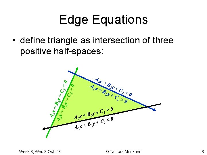
Edge Equations • define triangle as intersection of three positive half-spaces: Week 6, Wed 8 Oct 03 >0 3 +C 3 y +B A 3 x +B 3 y +C 3 <0 A 2 x +B +B 2 y 2 y +C +C 2 2 <0 >0 >0 C 1 + By A 1 x + 1 C 1 < 0 + y B A 1 x + 1 © Tamara Munzner 6

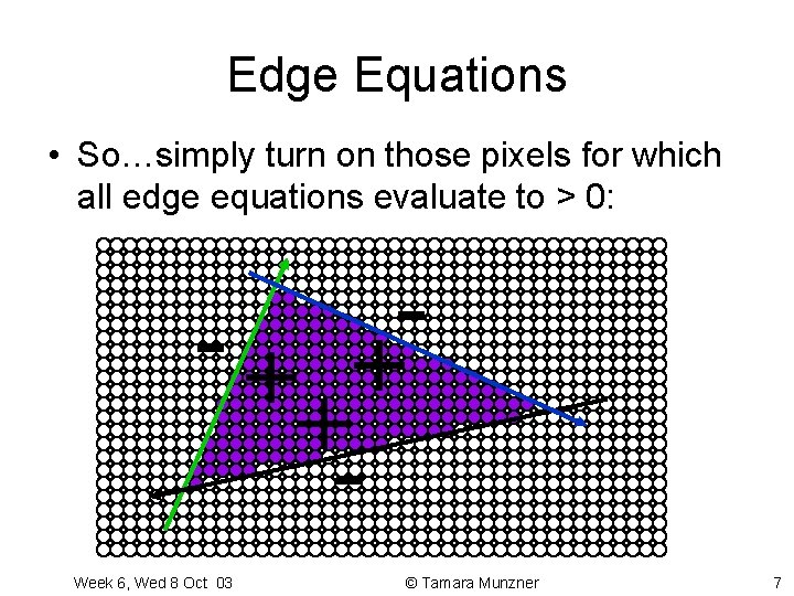
Edge Equations • So…simply turn on those pixels for which all edge equations evaluate to > 0: -+ + +Week 6, Wed 8 Oct 03 © Tamara Munzner 7

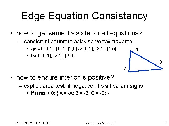
Edge Equation Consistency • how to get same +/- state for all equations? – consistent counterclockwise vertex traversal • good: [0, 1], [1, 2], [2, 0] or [0, 2], [2, 1], [1, 0] • bad: [0, 1], [2, 0] 1 0 2 • how to ensure interior is positive? – explicit area test: if negative, flip all param signs • if (area < 0) { A = -A; B = -B; C = -C; } Week 6, Wed 8 Oct 03 © Tamara Munzner 8

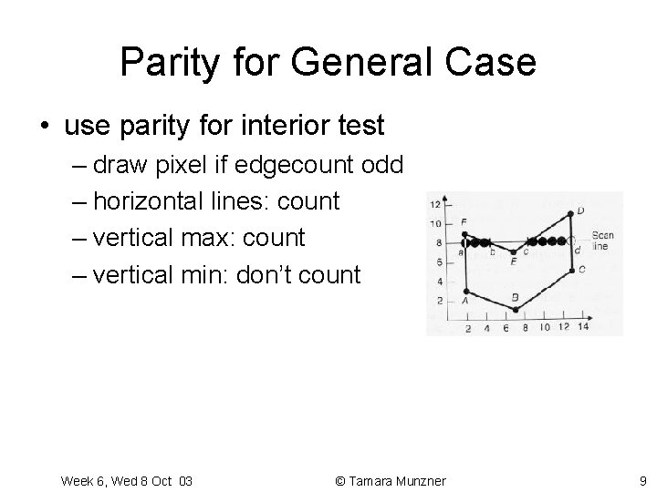
Parity for General Case • use parity for interior test – draw pixel if edgecount odd – horizontal lines: count – vertical max: count – vertical min: don’t count Week 6, Wed 8 Oct 03 © Tamara Munzner 9

Edge Tables • edge table (ET) – store edges sorted by y in linked list • at ymin, store ymax, xmin, slope • active edge table (AET) – active: currently used for computation – store active edges sorted by x • update each scanline, store ET values + current_x – for each scanline (from bottom to top) • do EAT bookkeeping • traverse EAT (from leftmost x to rightmost x) – draw pixels if parity odd Week 6, Wed 8 Oct 03 © Tamara Munzner 10

Edge Table Bookkeeping • setup: sorting in y – bucket sort, one bucket per pixel – add: simple check of ET[current_y] – delete edges if edge. ymax > current_y • main loop: sorting in x – for polygons that do not self-intersect, order of edges does not change between two scanlines – so insertion sort while adding new edges suffices Week 6, Wed 8 Oct 03 © Tamara Munzner 11

University of British Columbia CPSC 414 Computer Graphics Interpolation © Tamara Munzner 12

Scan Conversion • done: – how to determine pixels covered by a primitive • next: – how to assign pixel colors • interpolation of colors across triangles • interpolation of other properties Week 6, Wed 8 Oct 03 © Tamara Munzner 13

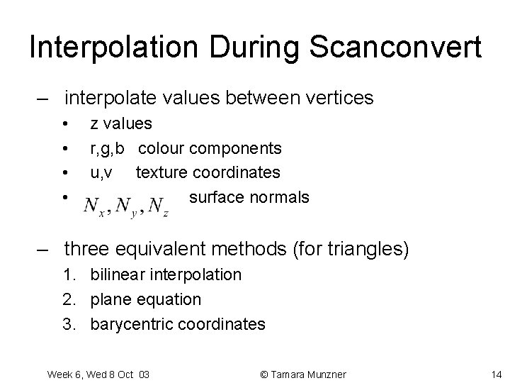
Interpolation During Scanconvert – interpolate values between vertices • • z values r, g, b colour components u, v texture coordinates surface normals – three equivalent methods (for triangles) 1. bilinear interpolation 2. plane equation 3. barycentric coordinates Week 6, Wed 8 Oct 03 © Tamara Munzner 14

1. Bilinear Interpolation – interpolate quantity along left-hand righthand edges, as a function of y • then interpolate quantity as a function of x – only triangles guarantee orientationindependent interpolation – compute efficiently by using known values at previous scanline, previous pixel Week 6, Wed 8 Oct 03 © Tamara Munzner 15

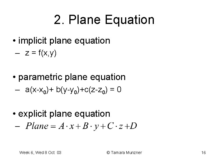
2. Plane Equation • implicit plane equation – z = f(x, y) • parametric plane equation – a(x-x 0)+ b(y-y 0)+c(z-z 0) = 0 • explicit plane equation – Week 6, Wed 8 Oct 03 © Tamara Munzner 16

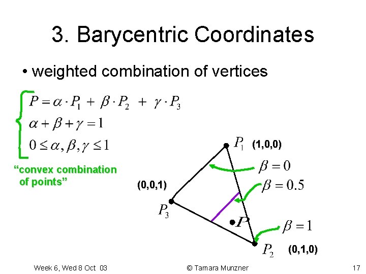
3. Barycentric Coordinates • weighted combination of vertices (1, 0, 0) “convex combination of points” (0, 0, 1) (0, 1, 0) Week 6, Wed 8 Oct 03 © Tamara Munzner 17

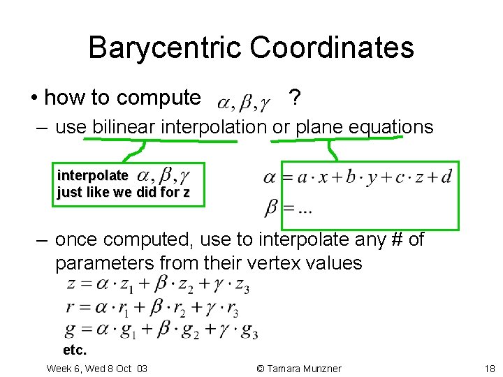
Barycentric Coordinates • how to compute ? – use bilinear interpolation or plane equations interpolate just like we did for z – once computed, use to interpolate any # of parameters from their vertex values etc. Week 6, Wed 8 Oct 03 © Tamara Munzner 18

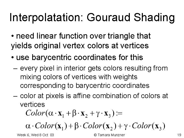
Interpolatation: Gouraud Shading • need linear function over triangle that yields original vertex colors at vertices • use barycentric coordinates for this – every pixel in interior gets colors resulting from mixing colors of vertices with weights corresponding to barycentric coordinates – color at pixels is affine combination of colors at vertices Week 6, Wed 8 Oct 03 © Tamara Munzner 19

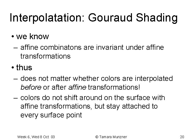
Interpolatation: Gouraud Shading • we know – affine combinatons are invariant under affine transformations • thus – does not matter whether colors are interpolated before or after affine transformations! – colors do not shift around on the surface with affine transformations, but stay attached to every surface point Week 6, Wed 8 Oct 03 © Tamara Munzner 20

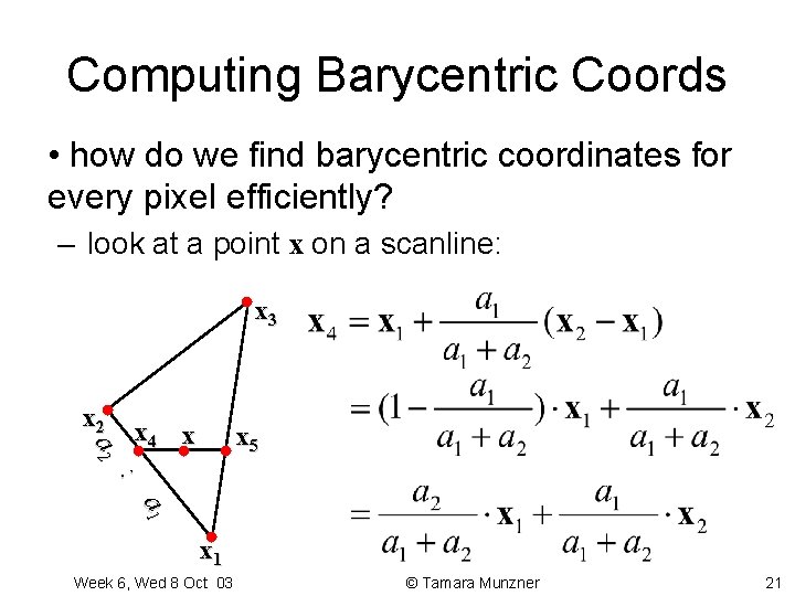
Computing Barycentric Coords • how do we find barycentric coordinates for every pixel efficiently? – look at a point x on a scanline: x 3 x 2 a 2 x 4 x x 5 : a 1 x 1 Week 6, Wed 8 Oct 03 © Tamara Munzner 21

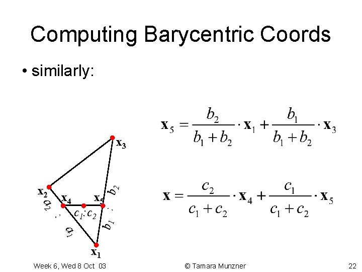
Computing Barycentric Coords • similarly: x 2 a 2 x 4 : x 5 c 1: c 2 a 1 b 1 : b 2 x 3 x 1 Week 6, Wed 8 Oct 03 © Tamara Munzner 22

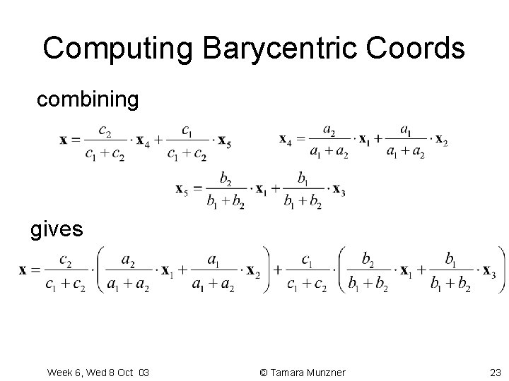
Computing Barycentric Coords combining gives Week 6, Wed 8 Oct 03 © Tamara Munzner 23

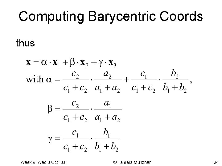
Computing Barycentric Coords thus Week 6, Wed 8 Oct 03 © Tamara Munzner 24

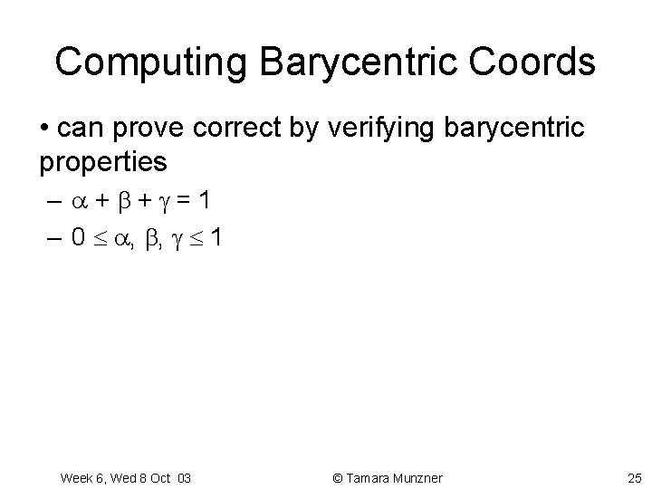
Computing Barycentric Coords • can prove correct by verifying barycentric properties – + + =1 – 0 , , 1 Week 6, Wed 8 Oct 03 © Tamara Munzner 25

Gouraud Shading with Bary Coords • algorithm – modify scanline algorithm for polygon scanconversion as follows: • linearly interpolate colors along edges of triangle to obtain colors for endpoints of span of pixels • linearly interpolate colors from these endpoints within the scanline Week 6, Wed 8 Oct 03 © Tamara Munzner 26

University of British Columbia CPSC 414 Computer Graphics Transforming Normals © Tamara Munzner 27

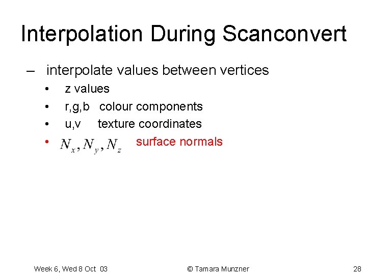
Interpolation During Scanconvert – interpolate values between vertices • • z values r, g, b colour components u, v texture coordinates surface normals Week 6, Wed 8 Oct 03 © Tamara Munzner 28

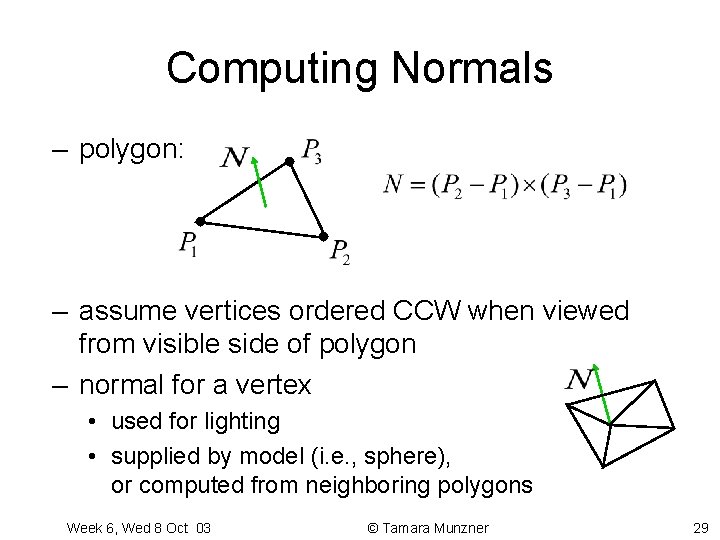
Computing Normals – polygon: – assume vertices ordered CCW when viewed from visible side of polygon – normal for a vertex • used for lighting • supplied by model (i. e. , sphere), or computed from neighboring polygons Week 6, Wed 8 Oct 03 © Tamara Munzner 29

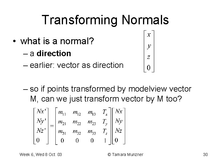
Transforming Normals • what is a normal? – a direction – earlier: vector as direction – so if points transformed by modelview vector M, can we just transform vector by M too? Week 6, Wed 8 Oct 03 © Tamara Munzner 30

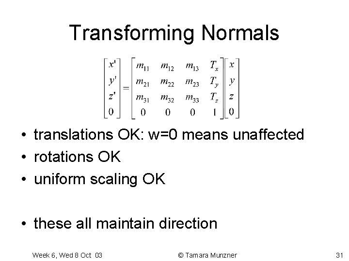
Transforming Normals • translations OK: w=0 means unaffected • rotations OK • uniform scaling OK • these all maintain direction Week 6, Wed 8 Oct 03 © Tamara Munzner 31

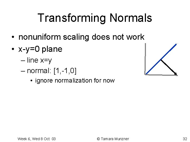
Transforming Normals • nonuniform scaling does not work • x-y=0 plane – line x=y – normal: [1, -1, 0] • ignore normalization for now Week 6, Wed 8 Oct 03 © Tamara Munzner 32

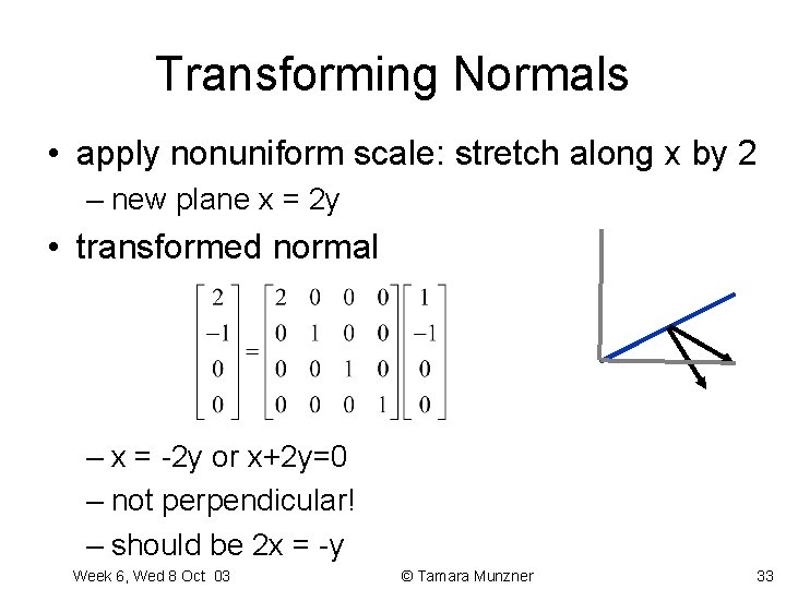
Transforming Normals • apply nonuniform scale: stretch along x by 2 – new plane x = 2 y • transformed normal – x = -2 y or x+2 y=0 – not perpendicular! – should be 2 x = -y Week 6, Wed 8 Oct 03 © Tamara Munzner 33

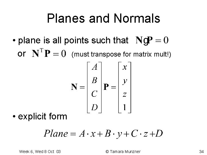
Planes and Normals • plane is all points such that or (must transpose for matrix mult!) • explicit form Week 6, Wed 8 Oct 03 © Tamara Munzner 34

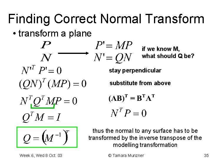
Finding Correct Normal Transform • transform a plane if we know M, what should Q be? stay perpendicular substitute from above thus the normal to any surface has to be transformed by the inverse transpose of the modelling transformation Week 6, Wed 8 Oct 03 © Tamara Munzner 35

University of British Columbia CPSC 414 Computer Graphics Sampling and Antialiasing © Tamara Munzner 36

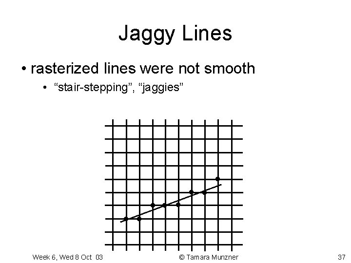
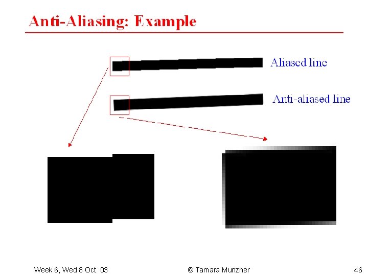
Jaggy Lines • rasterized lines were not smooth • “stair-stepping”, “jaggies” Week 6, Wed 8 Oct 03 © Tamara Munzner 37

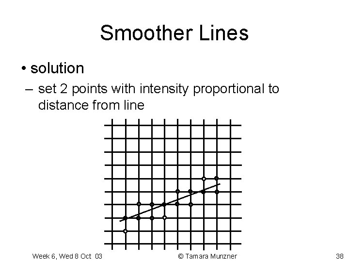
Smoother Lines • solution – set 2 points with intensity proportional to distance from line Week 6, Wed 8 Oct 03 © Tamara Munzner 38

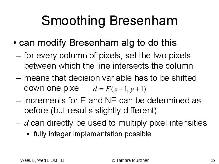
Smoothing Bresenham • can modify Bresenham alg to do this – for every column of pixels, set the two pixels between which the line intersects the column – means that decision variable has to be shifted down one pixel – increments for E and NE can be determined as before (but results slightly different) – d can directly be used to multiply pixel intensities • fully integer implementation possible Week 6, Wed 8 Oct 03 © Tamara Munzner 39

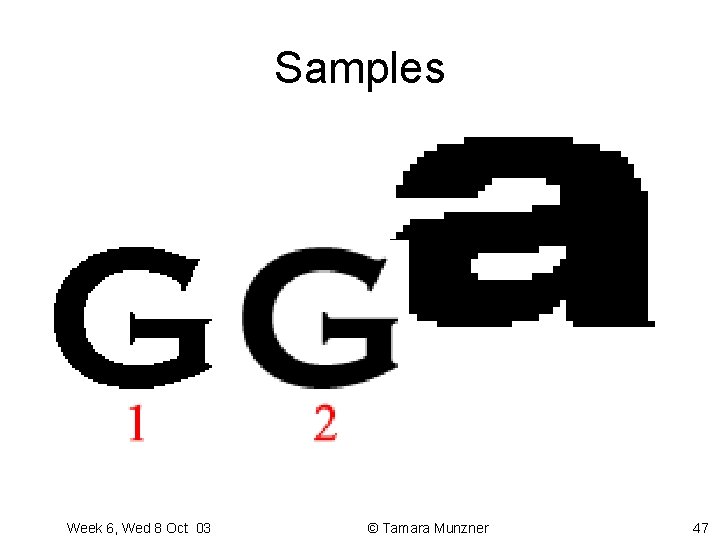
General Problem • “jaggies”: undesirable artifact – name for general problem is “aliasing” • solving the general problem – “antialiasing” • theoretical framework – sampling, signal processing Week 6, Wed 8 Oct 03 © Tamara Munzner 40

Samples • most things in the real world are continuous • everything in a computer is discrete • the process of mapping a continuous function to a discrete one is called sampling • the process of mapping a discrete function to a continuous one is called reconstruction • the process of mapping a continuous variable to a discrete one is called quantization • rendering an image requires sampling and quantization • displaying an image involves reconstruction Week 6, Wed 8 Oct 03 © Tamara Munzner 41

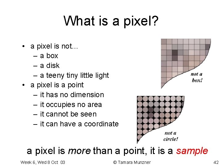
What is a pixel? • a pixel is not… – a box – a disk – a teeny tiny little light • a pixel is a point – it has no dimension – it occupies no area – it cannot be seen – it can have a coordinate a pixel is more than a point, it is a sample Week 6, Wed 8 Oct 03 © Tamara Munzner 42

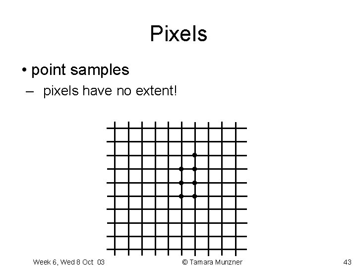
Pixels • point samples – pixels have no extent! Week 6, Wed 8 Oct 03 © Tamara Munzner 43

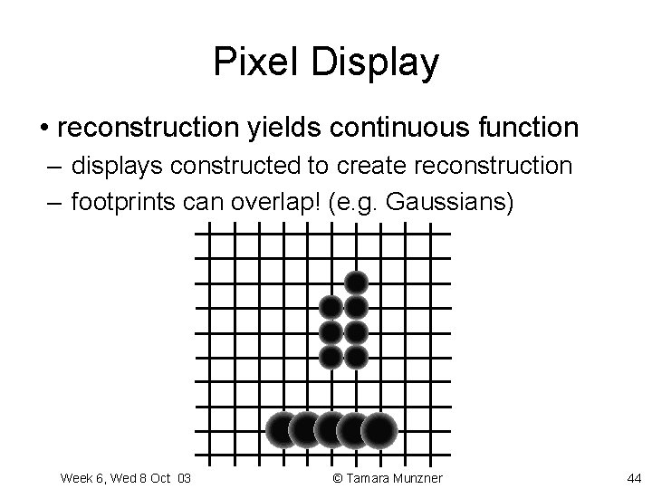
Pixel Display • reconstruction yields continuous function – displays constructed to create reconstruction – footprints can overlap! (e. g. Gaussians) Week 6, Wed 8 Oct 03 © Tamara Munzner 44

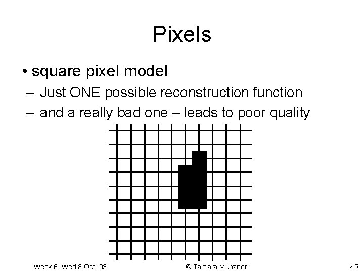
Pixels • square pixel model – Just ONE possible reconstruction function – and a really bad one – leads to poor quality Week 6, Wed 8 Oct 03 © Tamara Munzner 45

Samples Week 6, Wed 8 Oct 03 © Tamara Munzner 46

Samples Week 6, Wed 8 Oct 03 © Tamara Munzner 47

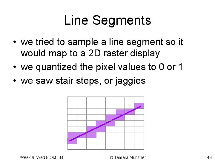
Line Segments • we tried to sample a line segment so it would map to a 2 D raster display • we quantized the pixel values to 0 or 1 • we saw stair steps, or jaggies Week 6, Wed 8 Oct 03 © Tamara Munzner 48

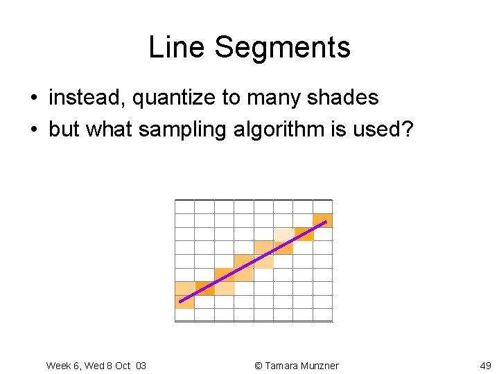
Line Segments • instead, quantize to many shades • but what sampling algorithm is used? Week 6, Wed 8 Oct 03 © Tamara Munzner 49

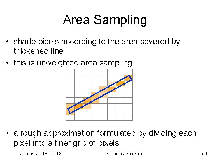
Area Sampling • shade pixels according to the area covered by thickened line • this is unweighted area sampling • a rough approximation formulated by dividing each pixel into a finer grid of pixels Week 6, Wed 8 Oct 03 © Tamara Munzner 50

Unweighted Area Sampling • primitive cannot affect intensity of pixel if it does not intersect the pixel • equal areas cause equal intensity, regardless of distance from pixel center to area Week 6, Wed 8 Oct 03 © Tamara Munzner 51

Weighted Area Sampling • unweighted sampling colors two pixels identically when the primitive cuts the same area through the two pixels • intuitively, pixel cut through the center should be more heavily weighted than one cut along corner Week 6, Wed 8 Oct 03 © Tamara Munzner 52

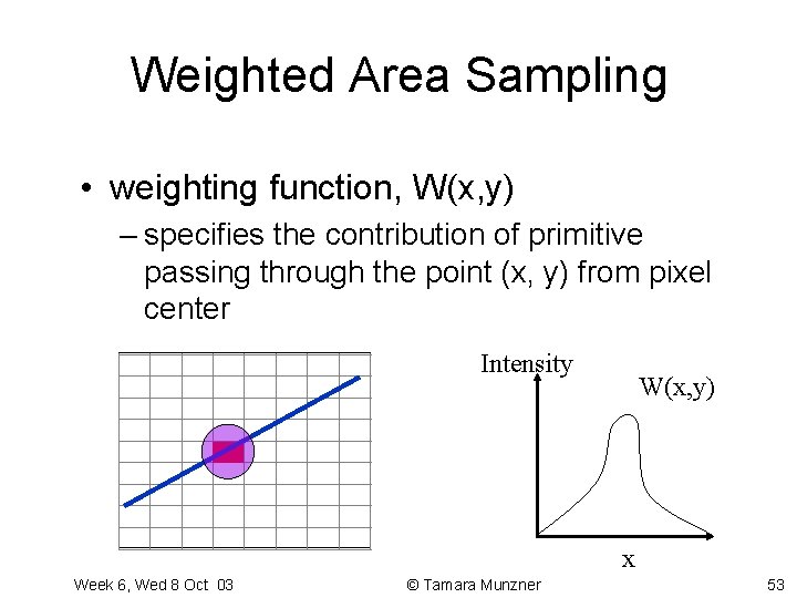
Weighted Area Sampling • weighting function, W(x, y) – specifies the contribution of primitive passing through the point (x, y) from pixel center Intensity W(x, y) x Week 6, Wed 8 Oct 03 © Tamara Munzner 53

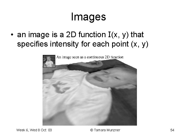
Images • an image is a 2 D function I(x, y) that specifies intensity for each point (x, y) Week 6, Wed 8 Oct 03 © Tamara Munzner 54

Sampling and Image • our goal is to convert the continuous image to a discrete set of samples • the graphics system’s display hardware will attempt to reconvert the samples into a continuous image: reconstruction Week 6, Wed 8 Oct 03 © Tamara Munzner 55

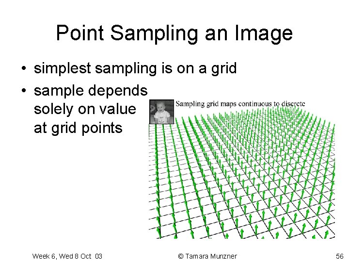
Point Sampling an Image • simplest sampling is on a grid • sample depends solely on value at grid points Week 6, Wed 8 Oct 03 © Tamara Munzner 56

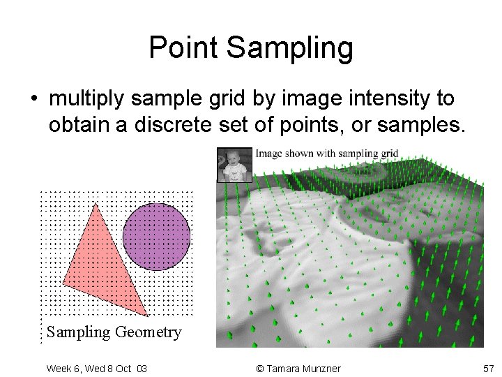
Point Sampling • multiply sample grid by image intensity to obtain a discrete set of points, or samples. Sampling Geometry Week 6, Wed 8 Oct 03 © Tamara Munzner 57

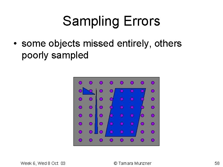
Sampling Errors • some objects missed entirely, others poorly sampled Week 6, Wed 8 Oct 03 © Tamara Munzner 58

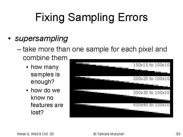
Fixing Sampling Errors • supersampling – take more than one sample for each pixel and combine them 150 x 15 to 100 x 10 • how many samples is enough? • how do we know no features are lost? Week 6, Wed 8 Oct 03 200 x 20 to 100 x 10 300 x 30 to 100 x 10 400 x 40 to 100 x 10 © Tamara Munzner 59