University of British Columbia CPSC 314 Computer Graphics

University of British Columbia CPSC 314 Computer Graphics Jan-Apr 2007 Tamara Munzner Procedural Approaches II, Picking Week 10, Wed Mar 21 • http: //www. ugrad. cs. ubc. ca/~cs 314/Vjan 2007

News • showing up for your project grading slot is not optional • 5 people have missed their slot, without notifying the TA in advance of the need to change • 2% penalty for noshows for P 3 and P 4 2

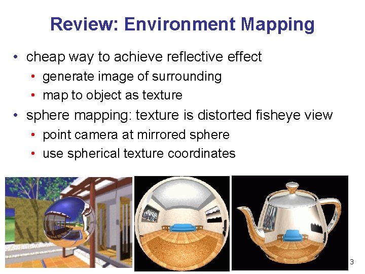
Review: Environment Mapping • cheap way to achieve reflective effect • generate image of surrounding • map to object as texture • sphere mapping: texture is distorted fisheye view • point camera at mirrored sphere • use spherical texture coordinates 3

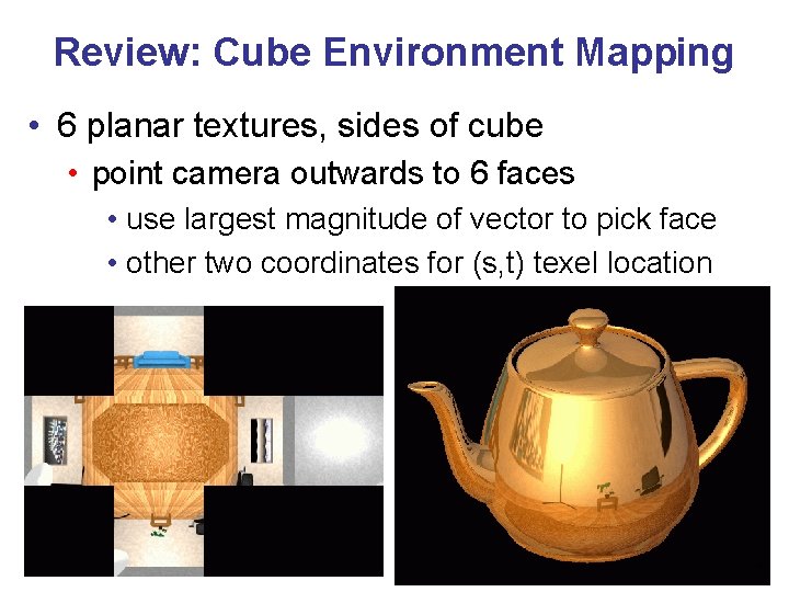
Review: Cube Environment Mapping • 6 planar textures, sides of cube • point camera outwards to 6 faces • use largest magnitude of vector to pick face • other two coordinates for (s, t) texel location 4

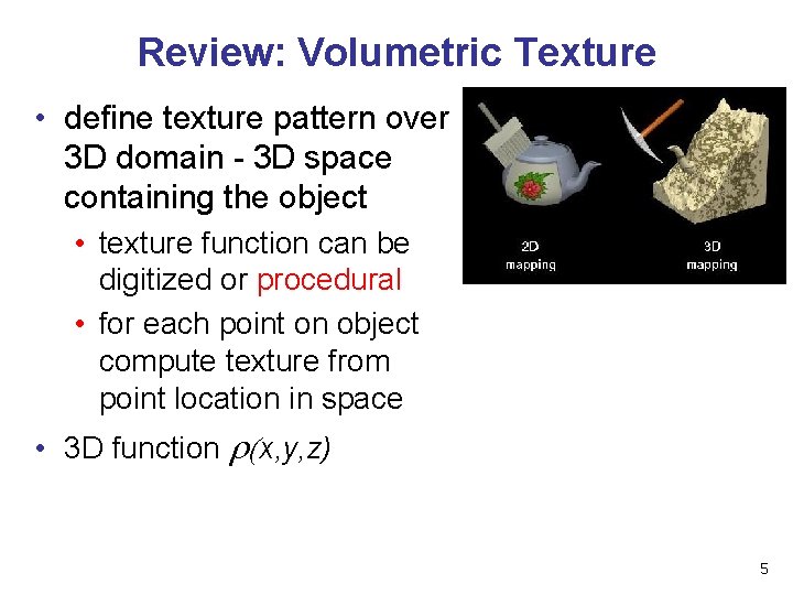
Review: Volumetric Texture • define texture pattern over 3 D domain - 3 D space containing the object • texture function can be digitized or procedural • for each point on object compute texture from point location in space • 3 D function r(x, y, z) 5

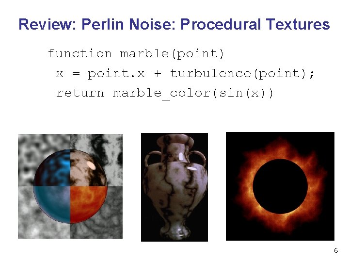
Review: Perlin Noise: Procedural Textures function marble(point) x = point. x + turbulence(point); return marble_color(sin(x)) 6

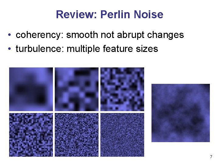
Review: Perlin Noise • coherency: smooth not abrupt changes • turbulence: multiple feature sizes 7

Review: Generating Coherent Noise • just three main ideas • nice interpolation • use vector offsets to make grid irregular • optimization • sneaky use of 1 D arrays instead of 2 D/3 D one 8

Review: Procedural Modeling • textures, geometry • nonprocedural: explicitly stored in memory • procedural approach • compute something on the fly • not load from disk • often less memory cost • visual richness • adaptable precision • noise, fractals, particle systems 9

Procedural Approaches II 10

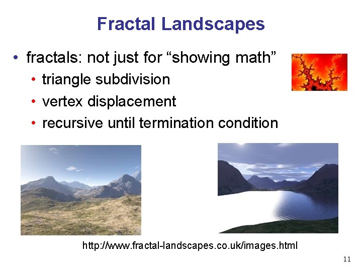
Fractal Landscapes • fractals: not just for “showing math” • triangle subdivision • vertex displacement • recursive until termination condition http: //www. fractal-landscapes. co. uk/images. html 11

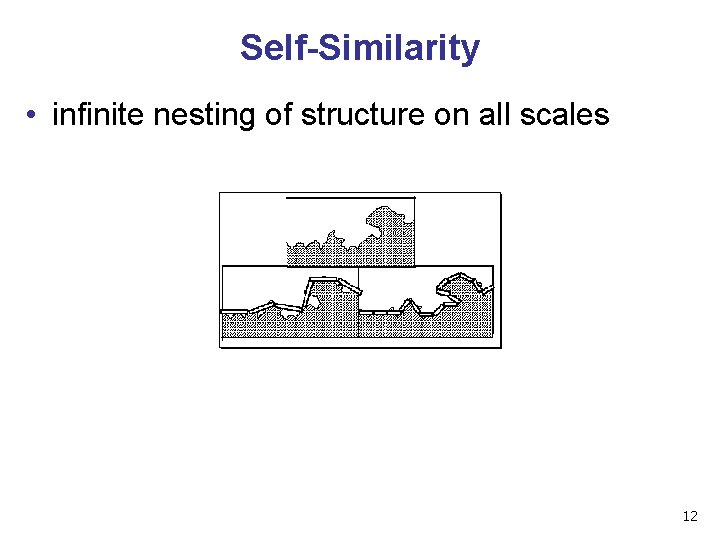
Self-Similarity • infinite nesting of structure on all scales 12

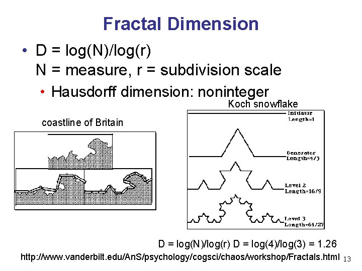
Fractal Dimension • D = log(N)/log(r) N = measure, r = subdivision scale • Hausdorff dimension: noninteger Koch snowflake coastline of Britain D = log(N)/log(r) D = log(4)/log(3) = 1. 26 http: //www. vanderbilt. edu/An. S/psychology/cogsci/chaos/workshop/Fractals. html 13

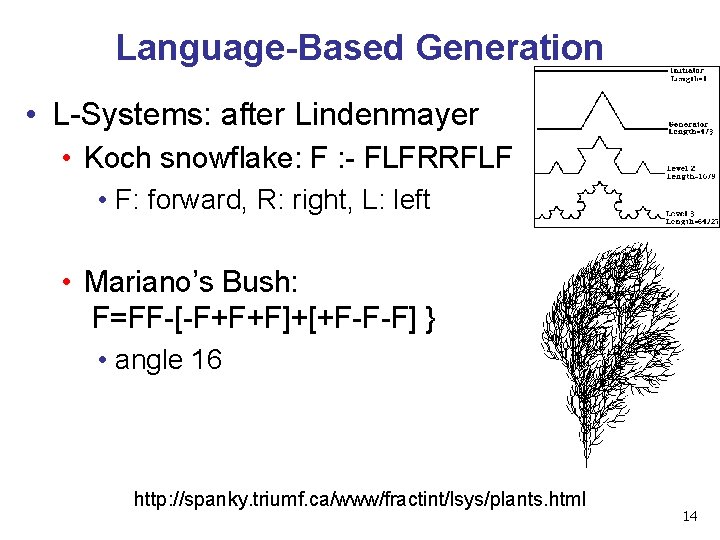
Language-Based Generation • L-Systems: after Lindenmayer • Koch snowflake: F : - FLFRRFLF • F: forward, R: right, L: left • Mariano’s Bush: F=FF-[-F+F+F]+[+F-F-F] } • angle 16 http: //spanky. triumf. ca/www/fractint/lsys/plants. html 14

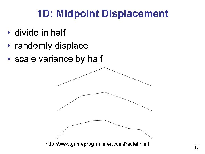
1 D: Midpoint Displacement • divide in half • randomly displace • scale variance by half http: //www. gameprogrammer. com/fractal. html 15

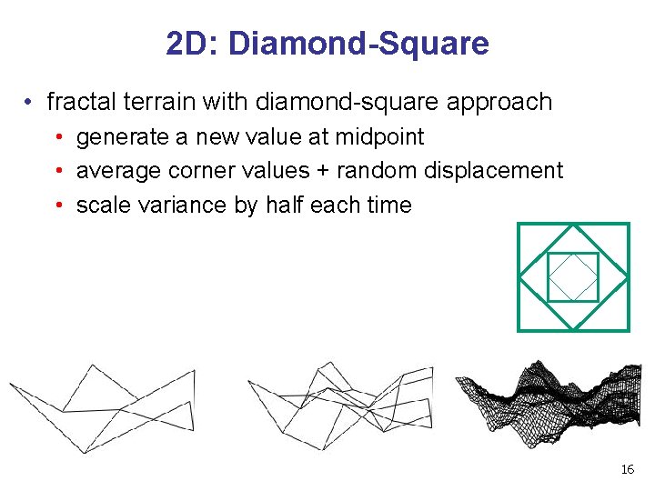
2 D: Diamond-Square • fractal terrain with diamond-square approach • generate a new value at midpoint • average corner values + random displacement • scale variance by half each time 16

Particle Systems • loosely defined • modeling, or rendering, or animation • key criteria • collection of particles • random element controls attributes • position, velocity (speed and direction), color, lifetime, age, shape, size, transparency • predefined stochastic limits: bounds, variance, type of distribution 17

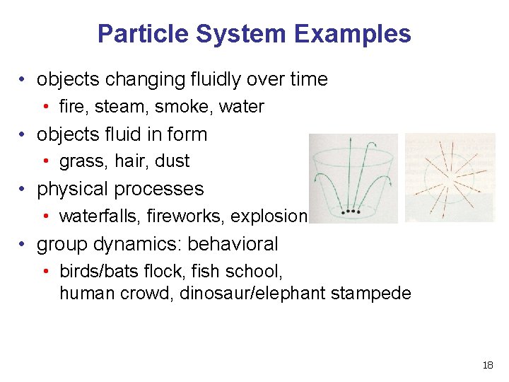
Particle System Examples • objects changing fluidly over time • fire, steam, smoke, water • objects fluid in form • grass, hair, dust • physical processes • waterfalls, fireworks, explosions • group dynamics: behavioral • birds/bats flock, fish school, human crowd, dinosaur/elephant stampede 18

Particle Systems Demos • general particle systems • http: //www. wondertouch. com • boids: bird-like objects • flocking/swarming behavior • procedural motion • http: //www. red 3 d. com/cwr/boids/ 19

Particle Life Cycle • generation • randomly within “fuzzy” location • initial attribute values: random or fixed • dynamics • attributes of each particle may vary over time • color darker as particle cools off after explosion • can also depend on other attributes • position: previous particle position + velocity + time • death • age and lifetime for each particle (in frames) • or if out of bounds, too dark to see, etc 20

Particle System Rendering • expensive to render thousands of particles • simplify: avoid hidden surface calculations • each particle has small graphical primitive (blob) • pixel color: sum of all particles mapping to it • some effects easy • temporal anti-aliasing (motion blur) • normally expensive: supersampling over time • position, velocity known for each particle • just render as streak 21

Procedural Approaches Summary • • Perlin noise fractals L-systems particle systems • not at all a complete list! • big subject: entire classes on this alone 22

Picking 23

Reading • Red Book • Selection and Feedback Chapter • all • Now That You Know Chapter • only Object Selection Using the Back Buffer 24

Interactive Object Selection • move cursor over object, click • how to decide what is below? • ambiguity • many 3 D world objects map to same 2 D point • four common approaches • manual ray intersection • bounding extents • backbuffer color coding • selection region with hit list 25

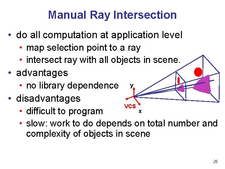
Manual Ray Intersection • do all computation at application level • map selection point to a ray • intersect ray with all objects in scene. • advantages • no library dependence y • disadvantages VCS x • difficult to program • slow: work to do depends on total number and complexity of objects in scene 26

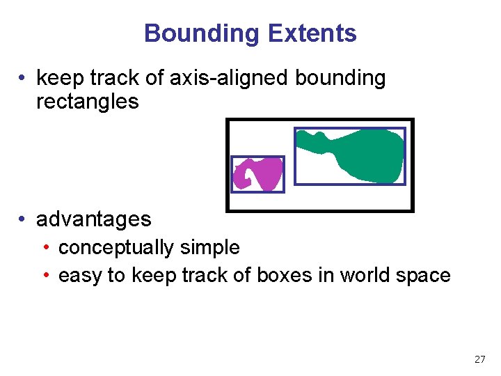
Bounding Extents • keep track of axis-aligned bounding rectangles • advantages • conceptually simple • easy to keep track of boxes in world space 27

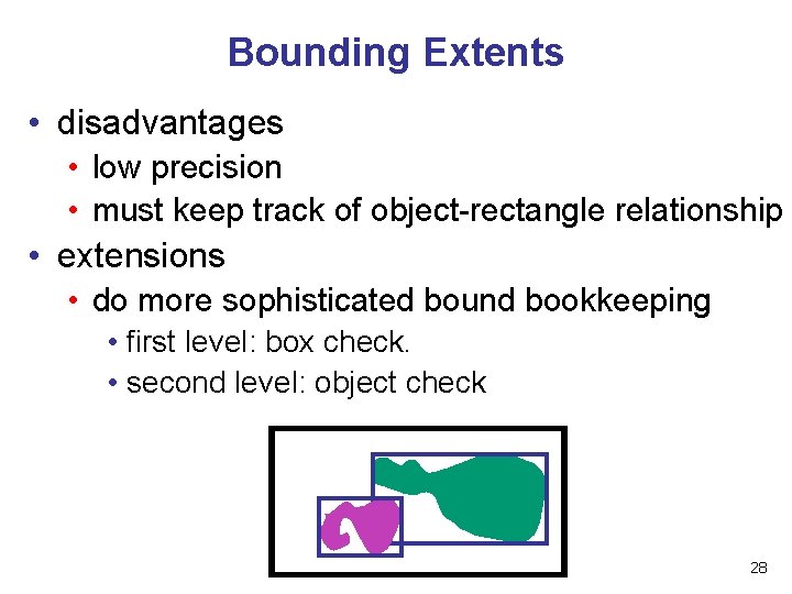
Bounding Extents • disadvantages • low precision • must keep track of object-rectangle relationship • extensions • do more sophisticated bound bookkeeping • first level: box check. • second level: object check 28

Backbuffer Color Coding • use backbuffer for picking • create image as computational entity • never displayed to user • redraw all objects in backbuffer • turn off shading calculations • set unique color for each pickable object • store in table • read back pixel at cursor location • check against table 29

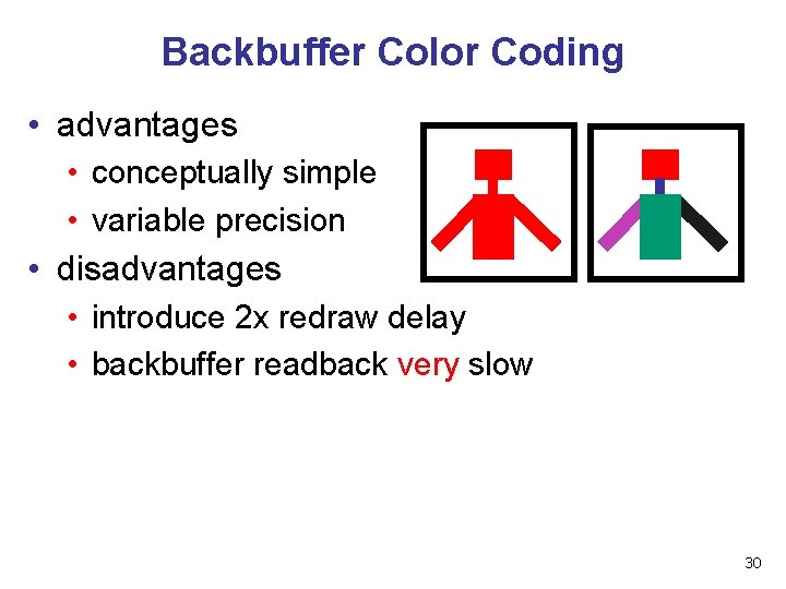
Backbuffer Color Coding • advantages • conceptually simple • variable precision • disadvantages • introduce 2 x redraw delay • backbuffer readback very slow 30

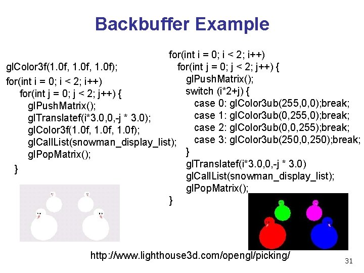
Backbuffer Example for(int i = 0; i < 2; i++) for(int j = 0; j < 2; j++) { gl. Color 3 f(1. 0 f, 1. 0 f); gl. Push. Matrix(); for(int i = 0; i < 2; i++) switch (i*2+j) { for(int j = 0; j < 2; j++) { case 0: gl. Color 3 ub(255, 0, 0); break; gl. Push. Matrix(); case 1: gl. Color 3 ub(0, 255, 0); break; gl. Translatef(i*3. 0, 0, -j * 3. 0); case 2: gl. Color 3 ub(0, 0, 255); break; gl. Color 3 f(1. 0 f, 1. 0 f); case 3: gl. Color 3 ub(250, 0, 250); break; gl. Call. List(snowman_display_list); } gl. Pop. Matrix(); gl. Translatef(i*3. 0, 0, -j * 3. 0) } gl. Call. List(snowman_display_list); gl. Pop. Matrix(); } http: //www. lighthouse 3 d. com/opengl/picking/ 31

Select/Hit • • • use small region around cursor for viewport assign per-object integer keys (names) redraw in special mode store hit list of objects in region examine hit list • Open. GL support 32

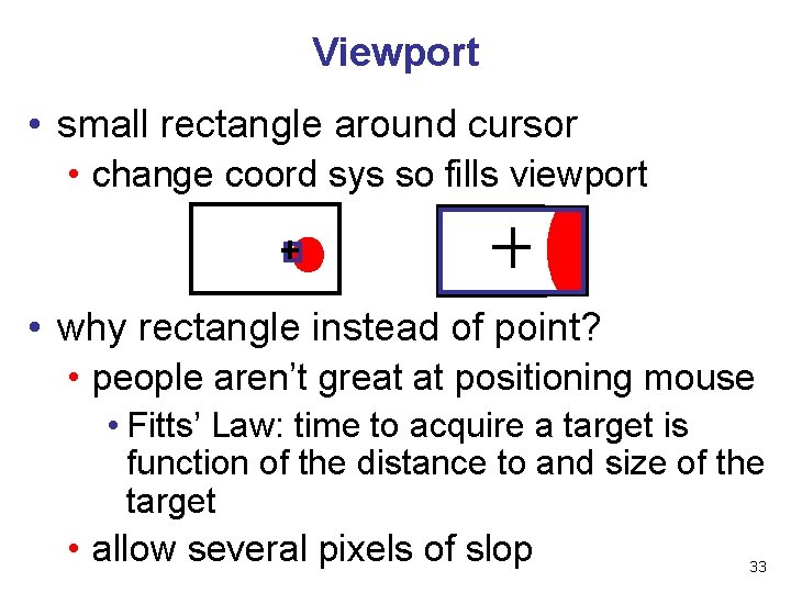
Viewport • small rectangle around cursor • change coord sys so fills viewport • why rectangle instead of point? • people aren’t great at positioning mouse • Fitts’ Law: time to acquire a target is function of the distance to and size of the target • allow several pixels of slop 33

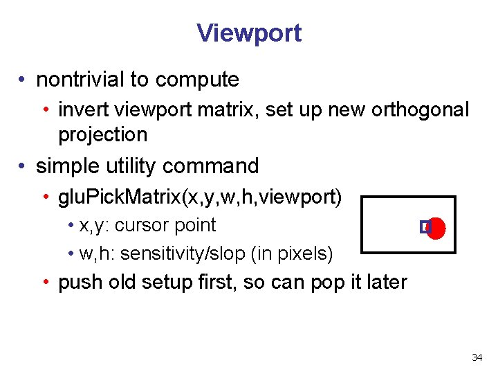
Viewport • nontrivial to compute • invert viewport matrix, set up new orthogonal projection • simple utility command • glu. Pick. Matrix(x, y, w, h, viewport) • x, y: cursor point • w, h: sensitivity/slop (in pixels) • push old setup first, so can pop it later 34

Render Modes • gl. Render. Mode(mode) • GL_RENDER: normal color buffer • default • GL_SELECT: selection mode for picking • (GL_FEEDBACK: report objects drawn) 35

Name Stack • again, "names" are just integers gl. Init. Names() • flat list gl. Load. Name(name) • or hierarchy supported by stack gl. Push. Name(name), gl. Pop. Name • can have multiple names per object 36

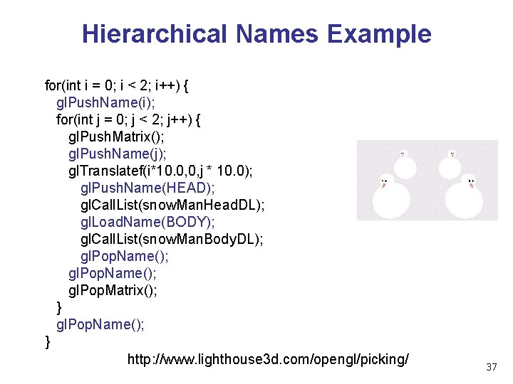
Hierarchical Names Example for(int i = 0; i < 2; i++) { gl. Push. Name(i); for(int j = 0; j < 2; j++) { gl. Push. Matrix(); gl. Push. Name(j); gl. Translatef(i*10. 0, 0, j * 10. 0); gl. Push. Name(HEAD); gl. Call. List(snow. Man. Head. DL); gl. Load. Name(BODY); gl. Call. List(snow. Man. Body. DL); gl. Pop. Name(); gl. Pop. Matrix(); } gl. Pop. Name(); } http: //www. lighthouse 3 d. com/opengl/picking/ 37

Hit List • gl. Select. Buffer(buffersize, *buffer) • where to store hit list data • on hit, copy entire contents of name stack to output buffer. • hit record • number of names on stack • minimum and minimum depth of object vertices • depth lies in the z-buffer range [0, 1] • multiplied by 2^32 -1 then rounded to nearest int 38

Integrated vs. Separate Pick Function • integrate: use same function to draw and pick • simpler to code • name stack commands ignored in render mode • separate: customize functions for each • potentially more efficient • can avoid drawing unpickable objects 39

Select/Hit • advantages • faster • Open. GL support means hardware acceleration • avoid shading overhead • flexible precision • size of region controllable • flexible architecture • custom code possible, e. g. guaranteed frame rate • disadvantages • more complex 40

Hybrid Picking • select/hit approach: fast, coarse • object-level granularity • manual ray intersection: slow, precise • exact intersection point • hybrid: both speed and precision • use select/hit to find object • then intersect ray with that object 41

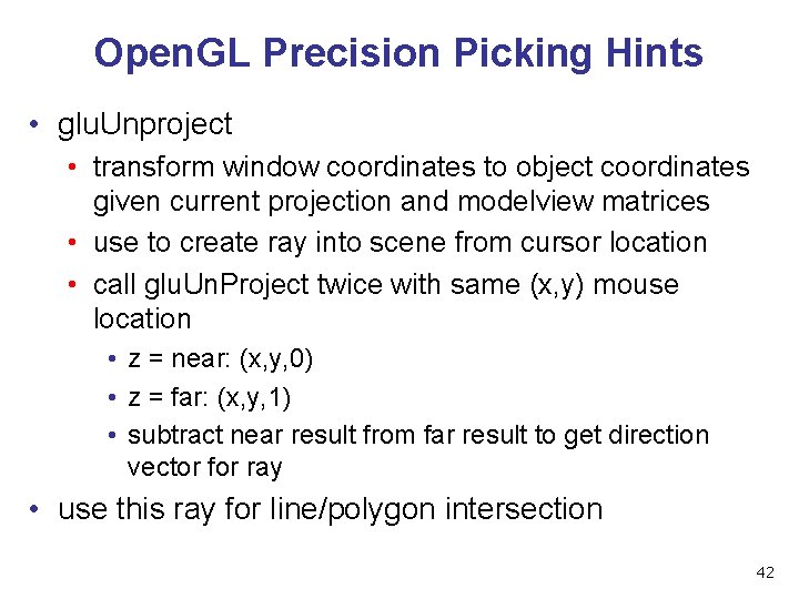
Open. GL Precision Picking Hints • glu. Unproject • transform window coordinates to object coordinates given current projection and modelview matrices • use to create ray into scene from cursor location • call glu. Un. Project twice with same (x, y) mouse location • z = near: (x, y, 0) • z = far: (x, y, 1) • subtract near result from far result to get direction vector for ray • use this ray for line/polygon intersection 42

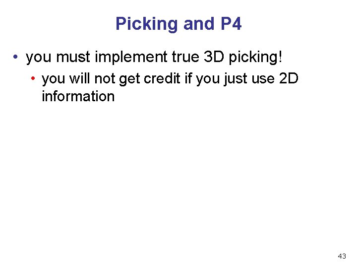
Picking and P 4 • you must implement true 3 D picking! • you will not get credit if you just use 2 D information 43