Universit di MilanoBicocca Laurea Magistrale in Informatica Corso

Università di Milano-Bicocca Laurea Magistrale in Informatica Corso di APPRENDIMENTO E APPROSSIMAZIONE Prof. Giancarlo Mauri Lezione 4 - Computational Learning Theory 1

Computational models of cognitive phenomena n Computing capabilities: Computability theory n Reasoning/deduction: n Learning/induction: Formal logic ? 2

A theory of the learnable (Valiant ‘ 84) n […] The problem is to discover good models that are interesting to study for their own sake and that promise to be relevant both to explaining human experience and to building devices that can learn […] Learning machines must have all 3 of the following properties: n the machines can provably learn whole classes of concepts, these classes can be characterized n the classes of concepts are appropriate and nontrivial for general-purpose knowledge n the computational process by which the machine builds the desired programs requires a “feasible” (i. e. polynomial) number of steps 3

A theory of the learnable n We seek general laws that constrain inductive learning, relating: n Probability of successful learning n Number of training examples n Complexity of hypothesis space n Accuracy to which target concept is approximated n Manner in which training examples are presented 4

Probably approximately correct learning formal computational model which want shed light on the limits of what can be learned by a machine, analysing the computational cost of learning algorithms 5

What we want to learn CONCEPT = recognizing algorithm LEARNING = computational description of recognizing algorithms starting from: - examples - incomplete specifications That is: to determine uniformly good approximations of an unknown function from its value in some sample points n interpolation n pattern matching n concept learning 6

What’s new in p. a. c. learning? Accuracy of results and running time for learning algorithms are explicitly quantified and related A general problem: use of resources (time, space…) by computations COMPLEXITY THEORY Example Sorting: n·logn time (polynomial, feasible) Bool. satisfiability: 2ⁿ time (exponential, intractable) 7

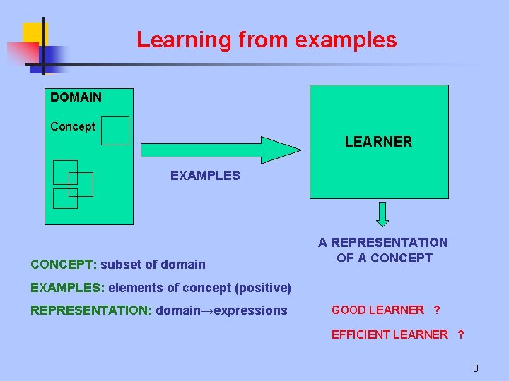
Learning from examples DOMAIN Concept LEARNER EXAMPLES CONCEPT: subset of domain A REPRESENTATION OF A CONCEPT EXAMPLES: elements of concept (positive) REPRESENTATION: domain→expressions GOOD LEARNER ? EFFICIENT LEARNER ? 8

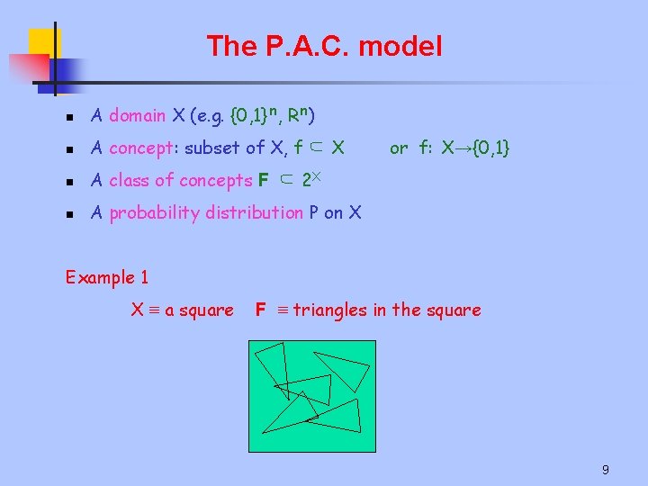
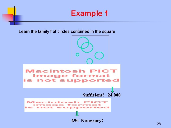
The P. A. C. model n A domain X (e. g. {0, 1}ⁿ, Rⁿ) n A concept: subset of X, f ⊆ X n A class of concepts F ⊆ 2 X n A probability distribution P on X or f: X→{0, 1} Example 1 X ≡ a square F ≡ triangles in the square 9

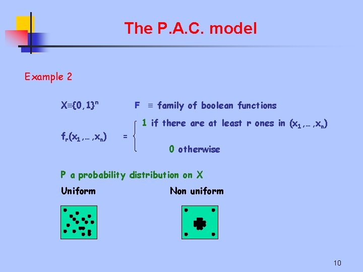
The P. A. C. model Example 2 X≡{0, 1}ⁿ fr(x 1, …, xn) F ≡ family of boolean functions = 1 if there at least r ones in (x 1, …, xn) 0 otherwise P a probability distribution on X Uniform Non uniform 10

The P. A. C. model The learning process n Labeled sample ((x 0, f(x 0)), (x 1, f(x 1)), …, (xn, f(xn)) n Hypothesis n Error probability a function h consistent with the sample (i. e. , h(xi) = f(xi) i) Perr(h(x)≠f(x), x X) 11

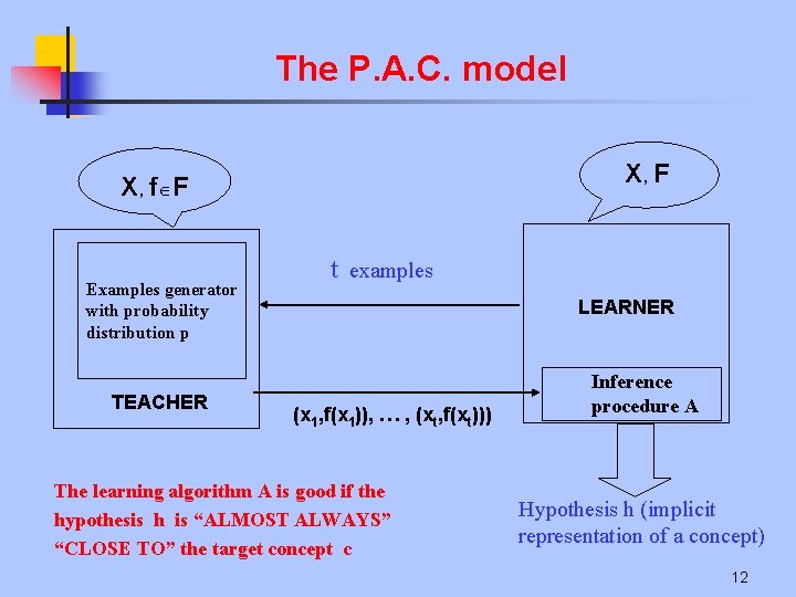
The P. A. C. model X, F X , f F Examples generator with probability distribution p TEACHER t examples LEARNER (x 1, f(x 1)), … , (xt, f(xt))) The learning algorithm A is good if the hypothesis h is “ALMOST ALWAYS” “CLOSE TO” the target concept c Inference procedure A Hypothesis h (implicit representation of a concept) 12

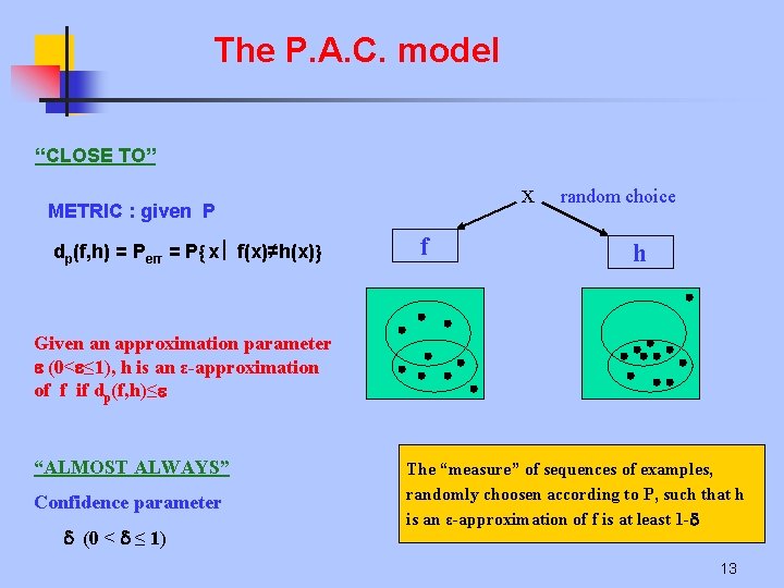
The P. A. C. model “CLOSE TO” x METRIC : given P dp(f, h) = Perr = P x f(x)≠h(x) f random choice h Given an approximation parameter (0< ≤ 1), h is an ε-approximation of f if dp(f, h)≤ “ALMOST ALWAYS” Confidence parameter (0 < ≤ 1) The “measure” of sequences of examples, randomly choosen according to P, such that h is an ε-approximation of f is at least 1 - 13

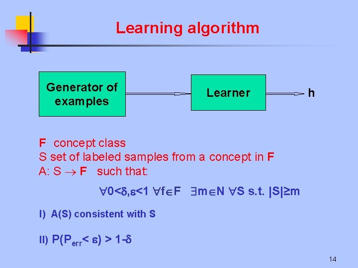
Learning algorithm Generator of examples Learner h F concept class S set of labeled samples from a concept in F A: S F such that: 0< , <1 f F m N S s. t. |S|≥m I) A(S) consistent with S II) P(Perr< ) > 1 - 14

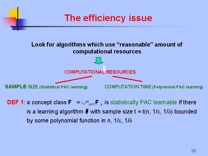
The efficiency issue Look for algorithms which use “reasonable” amount of computational resources COMPUTATIONAL RESOURCES SAMPLE SIZE (Statistical PAC learning) COMPUTATION TIME (Polynomial PAC learning) DEF 1: a concept class F = n=1 F n is statistically PAC learnable if there is a learning algorithm with sample size t = t(n, 1/ ) bounded by some polynomial function in n, 1/ 15

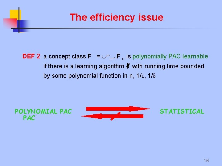
The efficiency issue DEF 2: a concept class F = n=1 F n is polynomially PAC learnable if there is a learning algorithm with running time bounded by some polynomial function in n, 1/ POLYNOMIAL PAC STATISTICAL 16

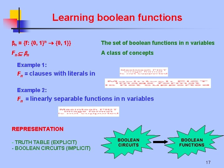
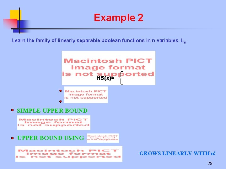
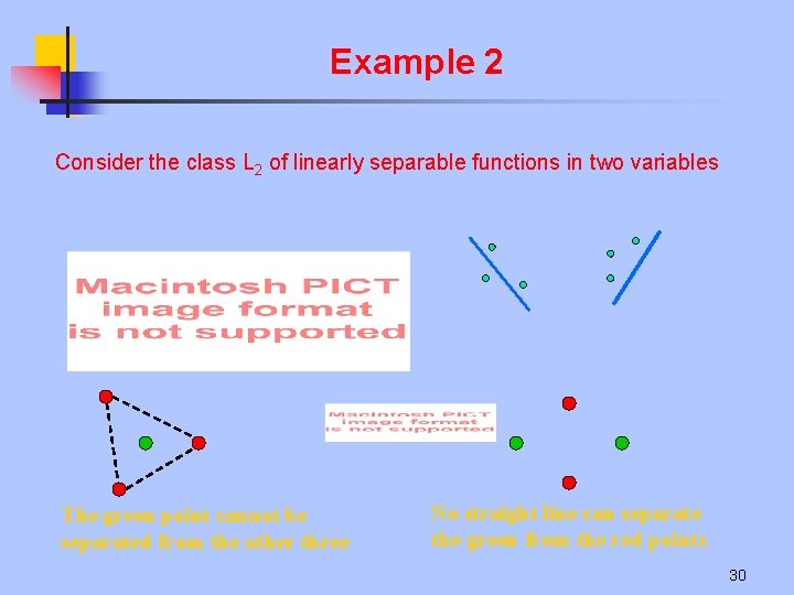
Learning boolean functions n = {f: {0, 1}n {0, 1}} The set of boolean functions in n variables Fn n A class of concepts Example 1: Fn = clauses with literals in Example 2: Fn = linearly separable functions in n variables REPRESENTATION - TRUTH TABLE (EXPLICIT) - BOOLEAN CIRCUITS (IMPLICIT) BOOLEAN CIRCUITS BOOLEAN FUNCTIONS 17

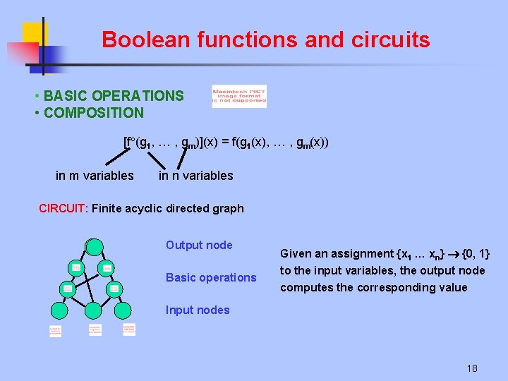
Boolean functions and circuits • BASIC OPERATIONS • COMPOSITION [f (g 1, … , gm)](x) = f(g 1(x), … , gm(x)) in m variables in n variables CIRCUIT: Finite acyclic directed graph Output node Basic operations Given an assignment {x 1 … xn} {0, 1} to the input variables, the output node computes the corresponding value Input nodes 18

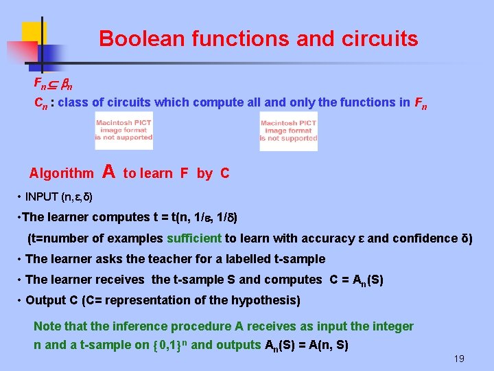
Boolean functions and circuits Fn n Cn : class of circuits which compute all and only the functions in Fn Algorithm A to learn F by C • INPUT (n, ε, δ) • The learner computes t = t(n, 1/ ) (t=number of examples sufficient to learn with accuracy ε and confidence δ) • The learner asks the teacher for a labelled t-sample • The learner receives the t-sample S and computes C = An(S) • Output C (C= representation of the hypothesis) Note that the inference procedure A receives as input the integer n and a t-sample on 0, 1 n and outputs An(S) = A(n, S) 19

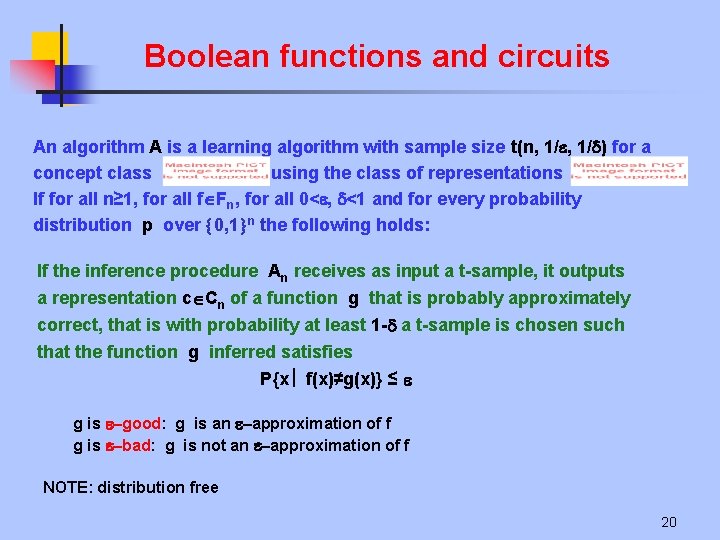
Boolean functions and circuits An algorithm A is a learning algorithm with sample size t(n, 1/ ) for a concept class using the class of representations If for all n≥ 1, for all f Fn, for all 0< , <1 and for every probability distribution p over 0, 1 n the following holds: If the inference procedure An receives as input a t-sample, it outputs a representation c Cn of a function g that is probably approximately correct, that is with probability at least 1 - a t-sample is chosen such that the function g inferred satisfies P{x f(x)≠g(x)} ≤ g is –good: g is an –approximation of f g is –bad: g is not an –approximation of f NOTE: distribution free 20

Statistical P. A. C. learning PROBLEM: Estimate upper and lower bounds on the sample size t = t(n, 1/ ) Upper bounds will be given for consistent algorithms Lower bounds will be given for arbitrary algorithms DEF: An inference procedure An for the class F n is consistent if, given the target function f F n, for every t-sample S = (<x 1, b 1>, … , <xt, bt>), An(S) is a representation of a function g “consistent” with S, i. e. g(x 1) = b 1, … , g(xt) = bt DEF: A learning algorithm A is consistent if its inference procedure is consistent 21

A simple upper bound THEOREM: t(n, 1/ ) ≤ -1 ln(#F n) +ln(1/ ) PROOF: Prob (x 1, … , xt) g (g(x 1)=f(x 1), … , g(xt)=f(xt) g -bad) ≤ ≤ g ε-bad P(AUB)≤P(A)+P(B) Prob (g(x 1) = f(x 1), … , g(xt) = f(xt)) ≤ Independent events Prob (g(xi) = f(xi)) g ε-bad i=1, … , t (1 - )t ≤ g ε-bad ≤ g is ε-bad #F n(1 - )t ≤ #F ne- t Impose #F n e- t ≤ NOTE - #F n must be finite 22

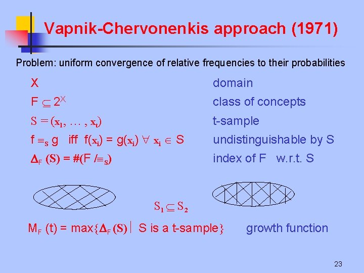
Vapnik-Chervonenkis approach (1971) Problem: uniform convergence of relative frequencies to their probabilities X domain F 2 X class of concepts S = (x 1, … , xt) t-sample f S g iff f(xi) = g(xi) xi S undistinguishable by S F (S) = #(F / S) index of F w. r. t. S S 1 S 2 MF (t) = max F (S) S is a t-sample growth function 23

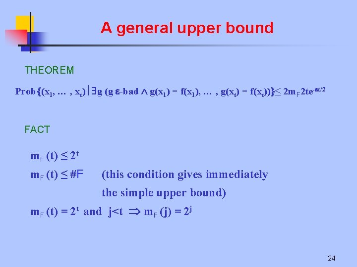
A general upper bound THEOREM Prob (x 1, … , xt) g (g -bad g(x 1) = f(x 1), … , g(xt) = f(xt)) ≤ 2 m. F 2 te- t/2 FACT m. F (t) ≤ 2 t m. F (t) ≤ #F (this condition gives immediately the simple upper bound) m. F (t) = 2 t and j<t m. F (j) = 2 j 24

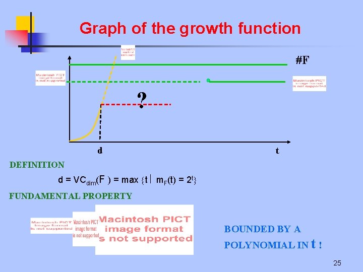
Graph of the growth function #F ? d t DEFINITION d = VCdim(F ) = max t m. F(t) = 2 t FUNDAMENTAL PROPERTY BOUNDED BY A POLYNOMIAL IN t ! 25

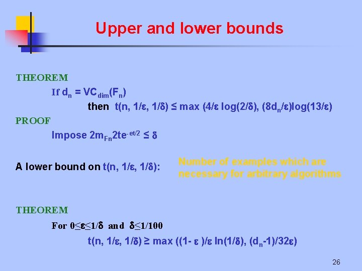
Upper and lower bounds THEOREM If dn = VCdim(Fn) then t(n, 1/ ) ≤ max (4/ log(2/ ), (8 dn/ )log(13/ ) PROOF Impose 2 m. Fn 2 te-et/2 ≤ A lower bound on t(n, 1/ ): Number of examples which are necessary for arbitrary algorithms THEOREM For 0≤ ≤ 1/ and ≤ 1/100 t(n, 1/ ) ≥ max ((1 - )/ ln(1/ ), (dn-1)/32 ) 26

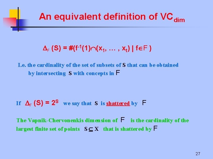
An equivalent definition of VCdim F (S) = #(f-1(1) (x 1, … , xt) | f F ) I. e. the cardinality of the set of subsets of S that can be obtained by intersecting S with concepts in F If F (S) = 2 S we say that S is shattered by F The Vapnik-Chervonenkis dimension of F is the cardinality of the largest finite set of points S X that is shattered by F 27

Example 1 Learn the family f of circles contained in the square Sufficient! 24. 000 690 Necessary! 28

Example 2 Learn the family of linearly separable boolean functions in n variables, Ln HS(x)= SIMPLE UPPER BOUND USING GROWS LINEARLY WITH n! 29

Example 2 Consider the class L 2 of linearly separable functions in two variables The green point cannot be separated from the other three No straight line can separate the green from the red points 30

Classi di formule booleane Monomi x 1 x 2 … xk DNF m 1 m 2 … mj (mj monomi) Clausole x 1 x 2 … xk CNF c 1 c 2 … cj k-DNF ≤ k letterali nei monomi k-term-DNF ≤ k monomi k-CNF ≤ k letterali nelle clausole k-clause-CNF ≤ k clausole Formule monotone non contengono letterali negati -formule ogni variabile appare al più una volta (cj clausole) 31

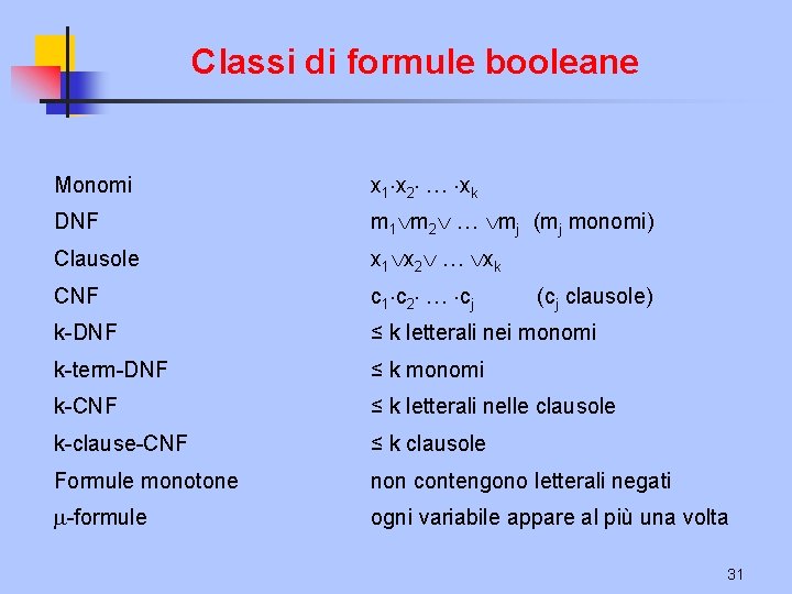
I risultati Th. (Valiant) I monomi sono apprendibili da esempi positivi con 2 (n+log ) esempi ( errore tollerato) ponendo in tutti gli es. N. B. L’apprendibilità è non monotona A B se B appr. , allora A appr. Th. i monomi non sono apprendibili da esempi negativi 32

Risultati positivi 1) K-CNF apprendibili da soli esempi positivi 1 b) K-DNF apprendibili da soli esempi negativi 2) (K-DNF K-CNF) apprendibili da es. (K-DNF K-CNF) positivi e negativi 3) la classe delle K-decision lists è apprendibile Th. Ogni K-DNF (o K-CNF)-formula è rappresentabile da una K-DL piccola 33

Risultati negativi 1) Le -formule non sono apprendibili 2) Le funzioni booleane a soglia non sono apprendibili 3) Per K ≥ 2, le formule K-term-DNF non sono apprendibili 34

Mistake bound model n So far: how many examples needed to learn ? n What about: how many mistakes before convergence ? n Let’s consider similar setting to PAC learning: n Instances drawn at random from X according to distribution D n Learner must classify each instance before receiving correct classification from teacher n Can we bound the number of mistakes learner makes before converging ? 35

Mistake bound model n Learner: n Receives a sequence of training examples x n Predicts the target value f(x) n Receives the correct target value from the trainer n Is evaluated by the total number of mistakes it makes before converging to the correct hypothesis n I. e. : n Learning takes place during the use of the system, not off-line n Ex. : prediction of fraudolent use of credit cards 36

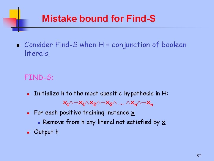
Mistake bound for Find-S n Consider Find-S when H = conjunction of boolean literals FIND-S: n Initialize h to the most specific hypothesis in H: x 1 x 2 … xn xn n For each positive training instance x n n Remove from h any literal not satisfied by x Output h 37

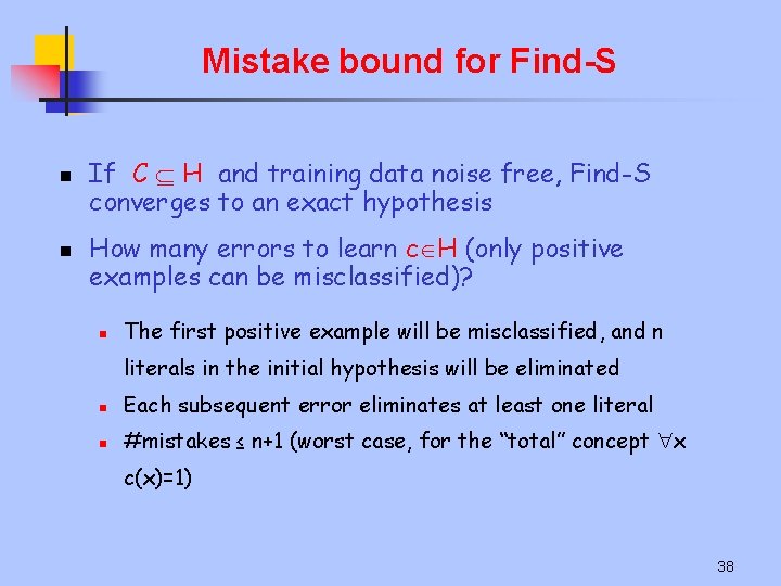
Mistake bound for Find-S n n If C H and training data noise free, Find-S converges to an exact hypothesis How many errors to learn c H (only positive examples can be misclassified)? n The first positive example will be misclassified, and n literals in the initial hypothesis will be eliminated n Each subsequent error eliminates at least one literal n #mistakes ≤ n+1 (worst case, for the “total” concept x c(x)=1) 38

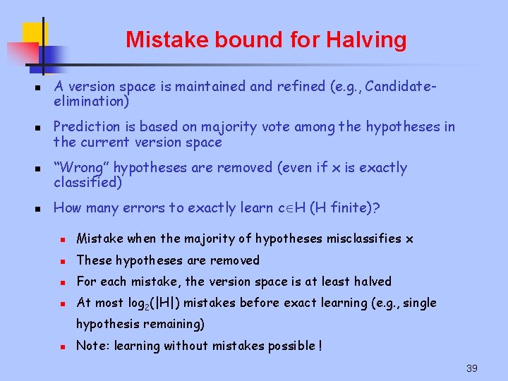
Mistake bound for Halving n n A version space is maintained and refined (e. g. , Candidateelimination) Prediction is based on majority vote among the hypotheses in the current version space “Wrong” hypotheses are removed (even if x is exactly classified) How many errors to exactly learn c H (H finite)? n Mistake when the majority of hypotheses misclassifies x n These hypotheses are removed n For each mistake, the version space is at least halved n At most log 2(|H|) mistakes before exact learning (e. g. , single hypothesis remaining) n Note: learning without mistakes possible ! 39

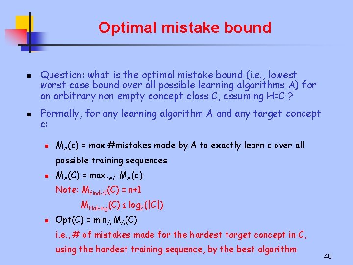
Optimal mistake bound n n Question: what is the optimal mistake bound (i. e. , lowest worst case bound over all possible learning algorithms A) for an arbitrary non empty concept class C, assuming H=C ? Formally, for any learning algorithm A and any target concept c: n MA(c) = max #mistakes made by A to exactly learn c over all possible training sequences n MA(C) = maxc C MA(c) Note: Mfind-S(C) = n+1 MHalving(C) ≤ log 2(|C|) n Opt(C) = min. A MA(C) i. e. , # of mistakes made for the hardest target concept in C, using the hardest training sequence, by the best algorithm 40

Optimal mistake bound n Theorem (Littlestone 1987) n VC(C) ≤ Opt(C) ≤ MHalving(C) ≤ log 2(|C|) n There exist concept classes for which VC(C) = Opt(C) = MHalving(C) = log 2(|C|) e. g. , the power set 2 X of X, for which it holds: VC(2 X) = |X| = log 2(|2 X|) n There exist concept classes for which n VC(C) < Opt(C) < MHalving(C) 41

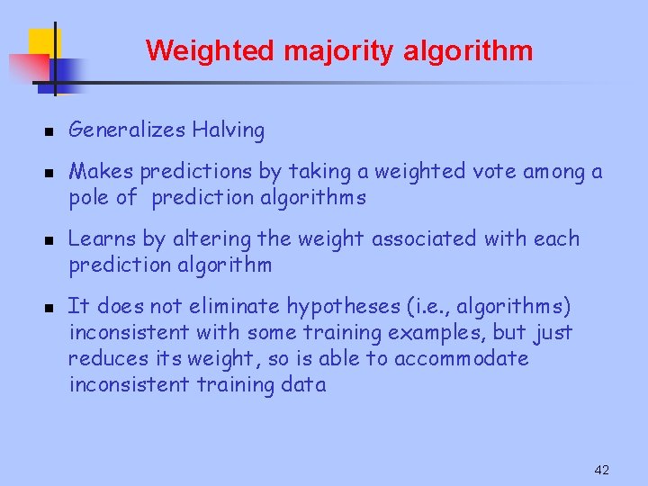
Weighted majority algorithm n n Generalizes Halving Makes predictions by taking a weighted vote among a pole of prediction algorithms Learns by altering the weight associated with each prediction algorithm It does not eliminate hypotheses (i. e. , algorithms) inconsistent with some training examples, but just reduces its weight, so is able to accommodate inconsistent training data 42

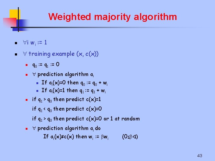
Weighted majority algorithm n i wi : = 1 n training example (x, c(x)) n q 0 : = q 1 : = 0 n prediction algorithm ai n n n If ai(x)=0 then q 0 : = q 0 + wi If ai(x)=1 then q 1 : = q 1 + wi if q 1 > q 0 then predict c(x)=1 if q 1 < q 0 then predict c(x)=0 if q 1 > q 0 then predict c(x)=0 or 1 at random n prediction algorithm ai do If ai(x)≠c(x) then wi : = wi (0≤ <1) 43

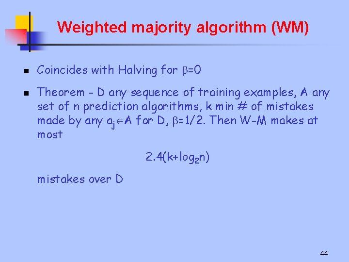
Weighted majority algorithm (WM) n n Coincides with Halving for =0 Theorem - D any sequence of training examples, A any set of n prediction algorithms, k min # of mistakes made by any aj A for D, =1/2. Then W-M makes at most 2. 4(k+log 2 n) mistakes over D 44

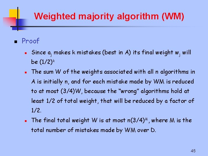
Weighted majority algorithm (WM) n Proof n Since aj makes k mistakes (best in A) its final weight wj will be (1/2)k n The sum W of the weights associated with all n algorithms in A is initially n, and for each mistake made by WM is reduced to at most (3/4)W, because the “wrong” algorithms hold at least 1/2 of total weight, that will be reduced by a factor of 1/2. n The final total weight W is at most n(3/4)M, where M is the total number of mistakes made by WM over D. 45

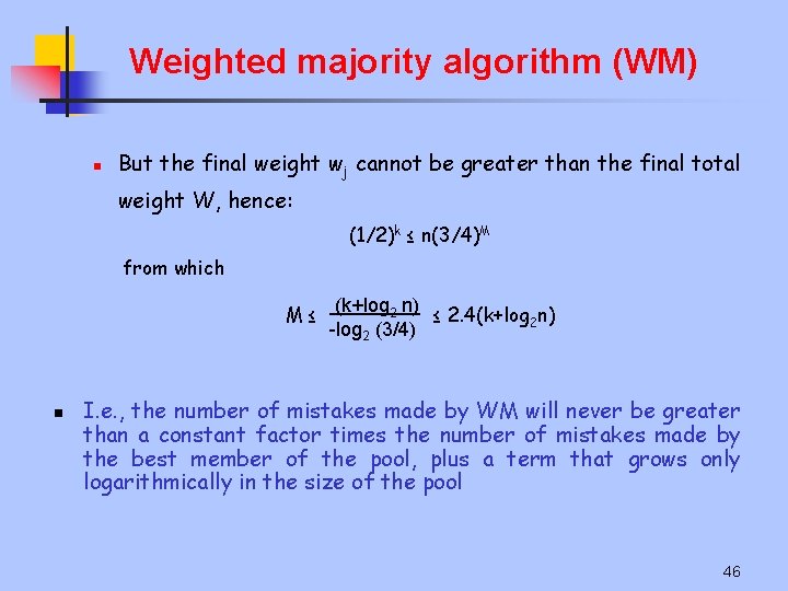
Weighted majority algorithm (WM) n But the final weight wj cannot be greater than the final total weight W, hence: (1/2)k ≤ n(3/4)M from which M≤ n (k+log 2 n) ≤ 2. 4(k+log 2 n) -log 2 (3/4) I. e. , the number of mistakes made by WM will never be greater than a constant factor times the number of mistakes made by the best member of the pool, plus a term that grows only logarithmically in the size of the pool 46