UNIVERSIT DEGLI STUDI DI SALERNO FACOLT DI INGEGNERIA

UNIVERSITÁ DEGLI STUDI DI SALERNO FACOLTÀ DI INGEGNERIA Bachelor Degree in Chemical Engineering Course: Process Instrumentation and Control (Strumentazione e Controllo dei Processi Chimici) REFERENCE LINEAR DYNAMIC SYSTEMS FIRST-ORDER PLUS DEAD TIME MODEL Rev. 3. 5 – May 17, 2019

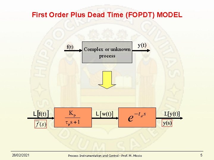
FIRST-ORDER PLUS DEAD TIME (FOPDT) MODEL f(t) Dead time Complex or unknown process w(t)=f(t-td) y(t) First order process y(t) This block representation provides a "frozen" picture of the dynamical system at a given time t 26/02/2021 Process Instrumentation and Control - Prof. M. Miccio 2

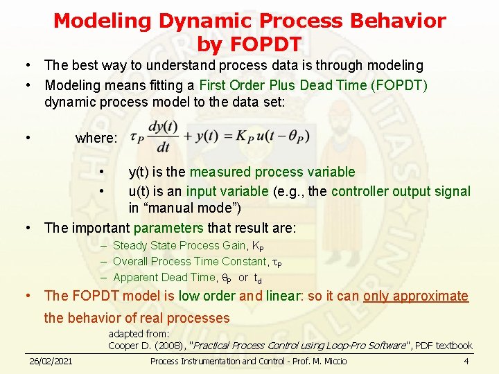
Modeling Dynamic Process Behavior by FOPDT • The best way to understand process data is through modeling • Modeling means fitting a First Order Plus Dead Time (FOPDT) dynamic process model to the data set: • where: • • y(t) is the measured process variable u(t) is an input variable (e. g. , the controller output signal in “manual mode”) • The important parameters that result are: – Steady State Process Gain, KP – Overall Process Time Constant, P – Apparent Dead Time, P or td • The FOPDT model is low order and linear: so it can only approximate the behavior of real processes adapted from: Cooper D. (2008), "Practical Process Control using Loop-Pro Software", PDF textbook 26/02/2021 Process Instrumentation and Control - Prof. M. Miccio 4

First Order Plus Dead Time (FOPDT) MODEL f(t) Complex or unknown process y(t) L[y(t)] 26/02/2021 Process Instrumentation and Control - Prof. M. Miccio 5

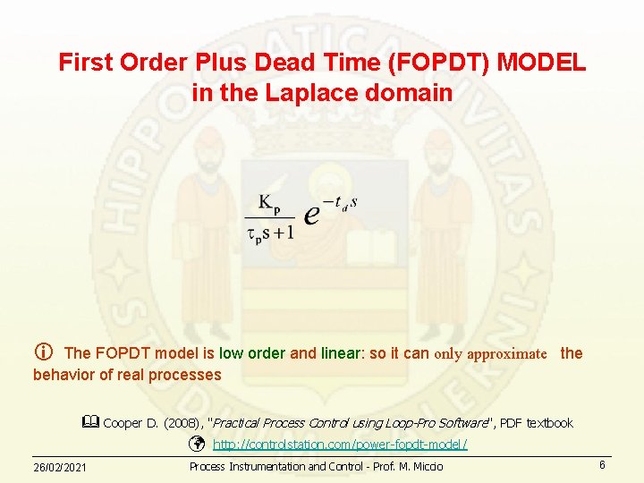
First Order Plus Dead Time (FOPDT) MODEL in the Laplace domain The FOPDT model is low order and linear: so it can only approximate the behavior of real processes Cooper D. (2008), "Practical Process Control using Loop-Pro Software", PDF textbook 26/02/2021 http: //controlstation. com/power-fopdt-model/ Process Instrumentation and Control - Prof. M. Miccio 6

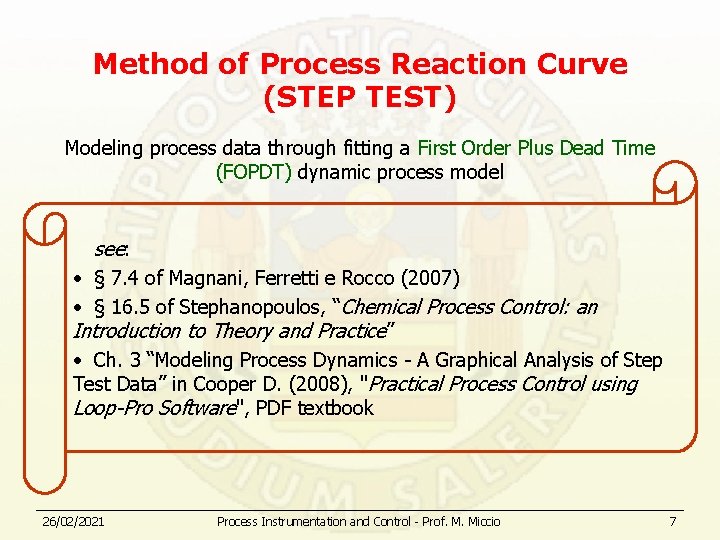
Method of Process Reaction Curve (STEP TEST) Modeling process data through fitting a First Order Plus Dead Time (FOPDT) dynamic process model see: • § 7. 4 of Magnani, Ferretti e Rocco (2007) • § 16. 5 of Stephanopoulos, “Chemical Process Control: an Introduction to Theory and Practice” • Ch. 3 “Modeling Process Dynamics - A Graphical Analysis of Step Test Data” in Cooper D. (2008), "Practical Process Control using Loop-Pro Software", PDF textbook 26/02/2021 Process Instrumentation and Control - Prof. M. Miccio 7

Fundamentals of Instrumentation & Process Control Two cases: 1. Self-regulating process 2. Non self-regulating process Copyright © 2006 Control Station, Inc. All Rights Reserved

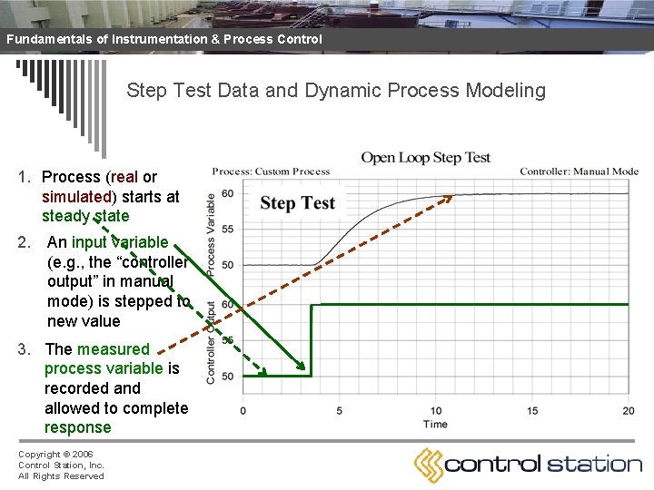
Fundamentals of Instrumentation & Process Control Step Test Data and Dynamic Process Modeling 1. Process (real or simulated) starts at steady state 2. An input variable (e. g. , the “controller output” in manual mode) is stepped to new value 3. The measured process variable is recorded and allowed to complete response Copyright © 2006 Control Station, Inc. All Rights Reserved

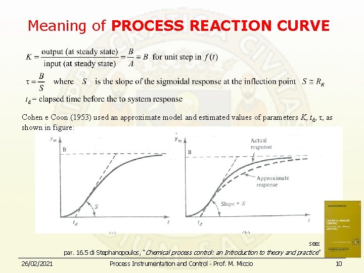
Meaning of PROCESS REACTION CURVE Cohen e Coon (1953) used an approximate model and estimated values of parameters K, td, τ, as shown in figure: see: par. 16. 5 di Stephanopoulos, “Chemical process control: an Introduction to theory and practice ” 26/02/2021 Process Instrumentation and Control - Prof. M. Miccio 10

Fundamentals of Instrumentation & Process Control Two cases: 1. Self-regulating process 2. Non self-regulating process Copyright © 2006 Control Station, Inc. All Rights Reserved

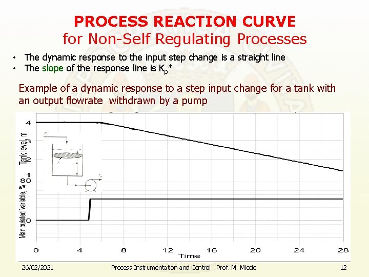
PROCESS REACTION CURVE for Non-Self Regulating Processes • The dynamic response to the input step change is a straight line • The slope of the response line is Kp* Example of a dynamic response to a step input change for a tank with an output flowrate withdrawn by a pump 26/02/2021 Process Instrumentation and Control - Prof. M. Miccio 12

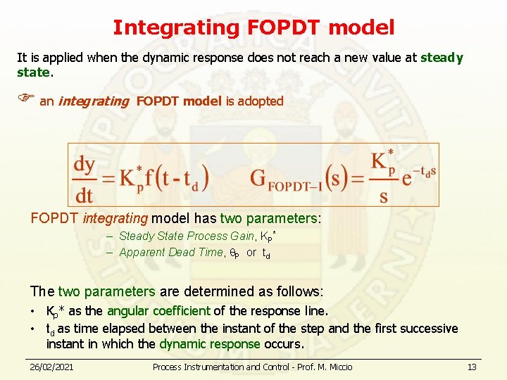
Integrating FOPDT model It is applied when the dynamic response does not reach a new value at steady state. an integrating FOPDT model is adopted FOPDT integrating model has two parameters: – Steady State Process Gain, KP* – Apparent Dead Time, P or td The two parameters are determined as follows: • Kp* as the angular coefficient of the response line. • td as time elapsed between the instant of the step and the first successive instant in which the dynamic response occurs. 26/02/2021 Process Instrumentation and Control - Prof. M. Miccio 13

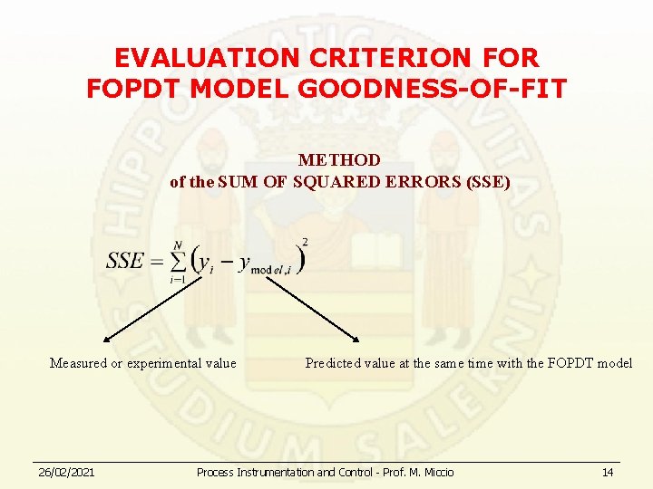
EVALUATION CRITERION FOR FOPDT MODEL GOODNESS-OF-FIT METHOD of the SUM OF SQUARED ERRORS (SSE) Measured or experimental value 26/02/2021 Predicted value at the same time with the FOPDT model Process Instrumentation and Control - Prof. M. Miccio 14

FOPDT MODEL PROCEDURE FOR THE CALCULATION OF PARAMETERS • SOFTWARE PROCEDURE • GRAPHICAL PROCEDURE • ANALYTICAL PROCEDURE 26/02/2021 Process Instrumentation and Control - Prof. M. Miccio 15

FOPDT MODEL PROCEDURE FOR THE CALCULATION OF PARAMETERS • SOFTWARE PROCEDURE • GRAPHICAL PROCEDURE • ANALYTICAL PROCEDURE 26/02/2021 Process Instrumentation and Control - Prof. M. Miccio 16

“Automatic” approximation to a first-order system and parameters estimation with the software LOOP-PRO • Available for response to the step test Øfor self-regulating system Øfor NON-inflected response Øfor inflected response • It requieres a file to record data of the response curve • It will be used for the students' Project Work • Download example files from: http: //comet. eng. unipr. it/~miccio/SCPC_it. htm#Control%20 Station 26/02/2021 Process Instrumentation and Control - Prof. M. Miccio 17

FOPDT MODEL PROCEDURE FOR THE CALCULATION OF PARAMETERS • SOFTWARE PROCEDURE • GRAPHICAL PROCEDURE • ANALYTICAL PROCEDURE 26/02/2021 Process Instrumentation and Control - Prof. M. Miccio 18

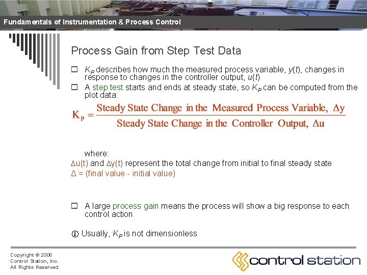
Fundamentals of Instrumentation & Process Control Process Gain from Step Test Data o KP describes how much the measured process variable, y(t), changes in response to changes in the controller output, u(t) o A step test starts and ends at steady state, so KP can be computed from the plot data: where: u(t) and y(t) represent the total change from initial to final steady state Δ = (final value - initial value) o A large process gain means the process will show a big response to each control action Usually, KP is not dimensionless Copyright © 2006 Control Station, Inc. All Rights Reserved

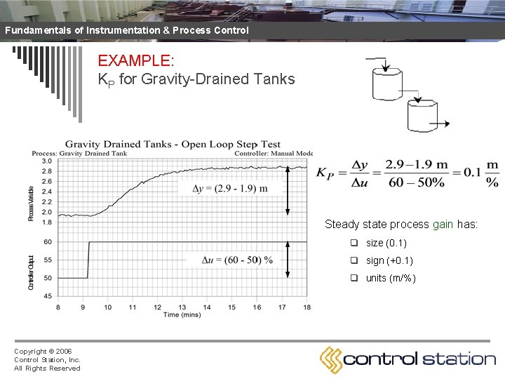
Fundamentals of Instrumentation & Process Control EXAMPLE: KP for Gravity-Drained Tanks Steady state process gain has: q size (0. 1) q sign (+0. 1) q units (m/%) Copyright © 2006 Control Station, Inc. All Rights Reserved

Fundamentals of Instrumentation & Process Control Time Constant and Dead Time from Step Test Data o They are computed from the plot of the measured process variable, y(t) o The calculation procedure may vary depending on n n Copyright © 2006 Control Station, Inc. All Rights Reserved the y(t) plot presents or doesn’t present an inflection point A software is used to minimize the model fitting error Calculation is graphically carried out directly on the plot Calculation is carried out by analytically using some data points on the plot

TIME CONSTANT and DEAD TIME from data of the step test Case N. 1 The curve responde does not show inflection point to the step test 26/02/2021 Process Instrumentation and Control - Prof. M. Miccio 22

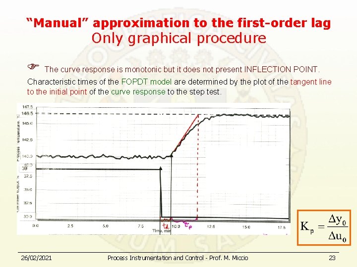
“Manual” approximation to the first-order lag Only graphical procedure The curve response is monotonic but it does not present INFLECTION POINT. Characteristic times of the FOPDT model are determined by the plot of the tangent line to the initial point of the curve response to the step test. 26/02/2021 Process Instrumentation and Control - Prof. M. Miccio 23

TIME CONSTANT and DEAD TIME from data of the step test Case N. 2 The curve response shows an inflection point to the step test (“sigmoidal” curve) 26/02/2021 Process Instrumentation and Control - Prof. M. Miccio 24

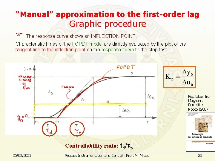
“Manual” approximation to the first-order lag Graphic procedure The response curve shows an INFLECTION POINT. Characteristic times of the FOPDT model are directly evaluated by the plot of the tangent line to the inflection point on the response curve to the step test. Fig. taken from Magnani, Ferretti e Rocco (2007) Controllability ratio: td/τp 26/02/2021 Process Instrumentation and Control - Prof. M. Miccio 25

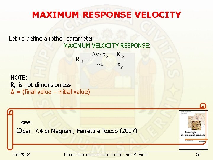
MAXIMUM RESPONSE VELOCITY Let us define another parameter: MAXIMUM VELOCITY RESPONSE: NOTE: RR is not dimensionless Δ = (final value – initial value) see: par. 7. 4 di Magnani, Ferretti e Rocco (2007) 26/02/2021 Process Instrumentation and Control - Prof. M. Miccio 26

FOPDT MODEL PROCEDURE FOR THE CALCULATION OF PARAMETERS • SOFTWARE PROCEDURE • GRAPHICAL PROCEDURE • ANALYTICAL PROCEDURE 26/02/2021 Process Instrumentation and Control - Prof. M. Miccio 27

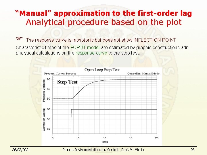
“Manual” approximation to the first-order lag Analytical procedure based on the plot The response curve is monotonic but does not show INFLECTION POINT. Characteristic times of the FOPDT model are estimated by graphic constructions adn analytical calculations on the response curve to the step test. 26/02/2021 Process Instrumentation and Control - Prof. M. Miccio 28

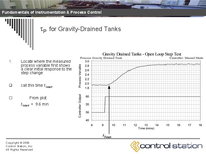
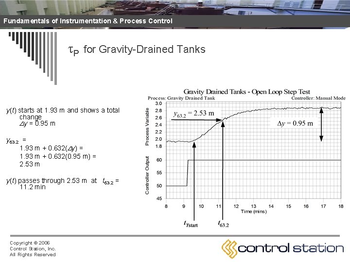
Fundamentals of Instrumentation & Process Control P for Gravity-Drained Tanks 1. Locate where the measured process variable first shows a clear initial response to the step change q call this time t. Ystart o From plot: t. Ystart = 9. 6 min Copyright © 2006 Control Station, Inc. All Rights Reserved

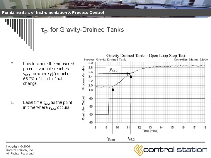
Fundamentals of Instrumentation & Process Control P for Gravity-Drained Tanks 2. Locate where the measured process variable reaches y 63. 2, or where y(t) reaches 63. 2% of its total final change o Label time t 63. 2 as the point in time where y 63. 2 occurs Copyright © 2006 Control Station, Inc. All Rights Reserved

Fundamentals of Instrumentation & Process Control P for Gravity-Drained Tanks y(t) starts at 1. 93 m and shows a total change y = 0. 95 m y 63. 2 = 1. 93 m + 0. 632( y) = 1. 93 m + 0. 632(0. 95 m) = 2. 53 m y(t) passes through 2. 53 m at t 63. 2 = 11. 2 min Copyright © 2006 Control Station, Inc. All Rights Reserved

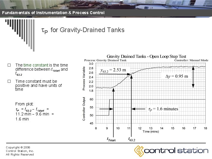
Fundamentals of Instrumentation & Process Control P for Gravity-Drained Tanks o The time constant is the time difference between t. Ystart and t 63. 2 o Time constant must be positive and have units of time From plot: P = t 63. 2 t. Ystart = 11. 2 min 9. 6 min = 1. 6 min Copyright © 2006 Control Station, Inc. All Rights Reserved

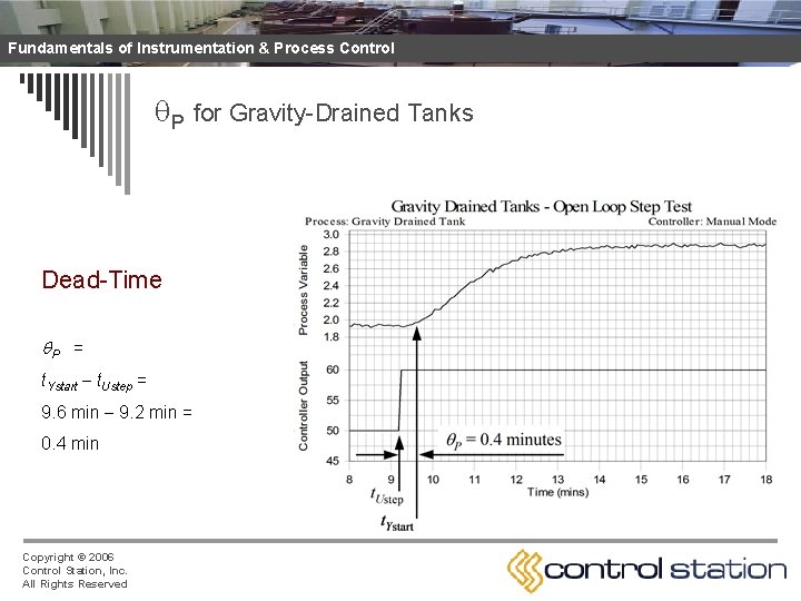
Fundamentals of Instrumentation & Process Control Apparent Dead-Time from Step Test Data o P is the time from when the controller output step is made until when the measured process variable first responds o Apparent dead time, P, is the sum of these effects: n transportation lag, or the time it takes for material to travel from one point to another n sample or instrument lag, or the time it takes to collect analyze or process a measured variable sample n higher order processes naturally appear slow to respond o Notes: n Dead time must be positive and have units of time n Tight control in increasingly difficult as P P n For important loops, work to avoid unnecessary dead time Copyright © 2006 Control Station, Inc. All Rights Reserved

Fundamentals of Instrumentation & Process Control P for Gravity-Drained Tanks Dead-Time P = t. Ystart t. Ustep = 9. 6 min 9. 2 min = 0. 4 min Copyright © 2006 Control Station, Inc. All Rights Reserved

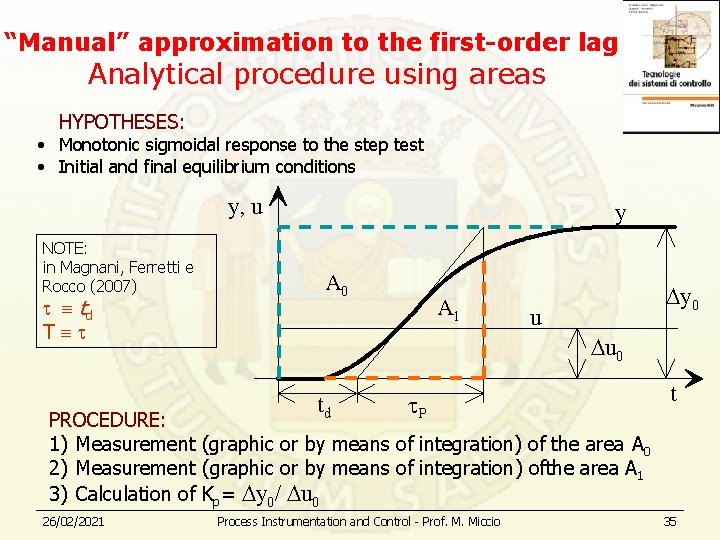
“Manual” approximation to the first-order lag Analytical procedure using areas HYPOTHESES: • Monotonic sigmoidal response to the step test • Initial and final equilibrium conditions y, u NOTE: in Magnani, Ferretti e Rocco (2007) td T y A 0 A 1 y 0 u u 0 td P t PROCEDURE: 1) Measurement (graphic or by means of integration) of the area A 0 2) Measurement (graphic or by means of integration) ofthe area A 1 3) Calculation of Kp= y 0/ u 0 26/02/2021 Process Instrumentation and Control - Prof. M. Miccio 35

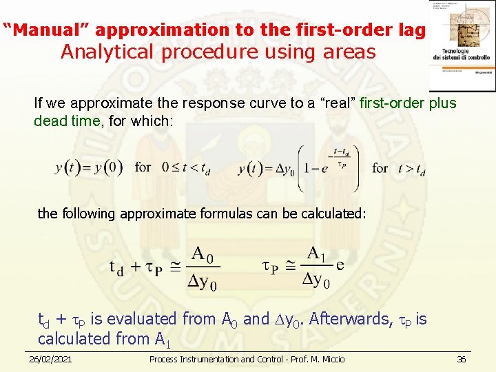
“Manual” approximation to the first-order lag Analytical procedure using areas If we approximate the response curve to a “real” first-order plus dead time, for which: the following approximate formulas can be calculated: td + P is evaluated from A 0 and y 0. Afterwards, P is calculated from A 1 26/02/2021 Process Instrumentation and Control - Prof. M. Miccio 36