Univariate Statistics Analysis of a single variable Two

Univariate Statistics • Analysis of a single variable • Two general varieties: • Descriptive Statistics: Describe Variables (where data are any collection of observations, sample/population) • Inferential Statistics: Make inferences about the population based on characteristics of sample data

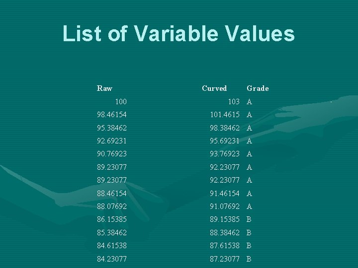
List of Variable Values Raw Curved Grade 100 103 A 98. 46154 101. 4615 A 95. 38462 98. 38462 A 92. 69231 95. 69231 A 90. 76923 93. 76923 A 89. 23077 92. 23077 A 88. 46154 91. 46154 A 88. 07692 91. 07692 A 86. 15385 89. 15385 B 85. 38462 88. 38462 B 84. 61538 87. 61538 B 84. 23077 87. 23077 B

Frequency Distribution • A summary of the observations for a variable • Includes a list of the values of the variable and the frequency of observations for each value

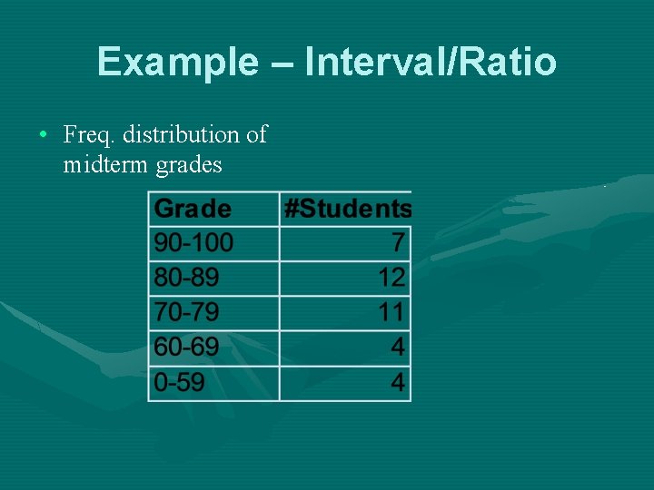
Example – Interval/Ratio • Freq. distribution of midterm grades

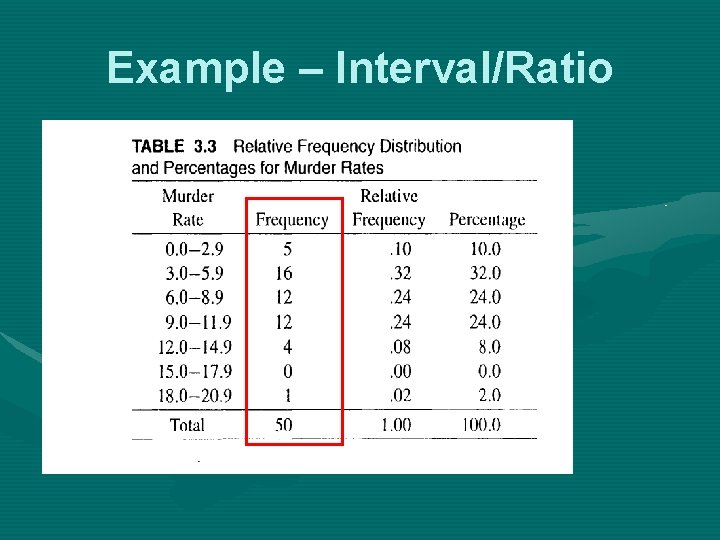
Example – Interval/Ratio

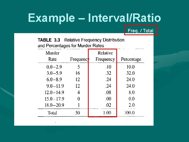
Example – Interval/Ratio Freq. / Total

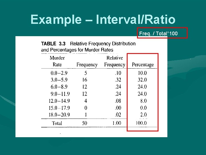
Example – Interval/Ratio Freq. / Total*100

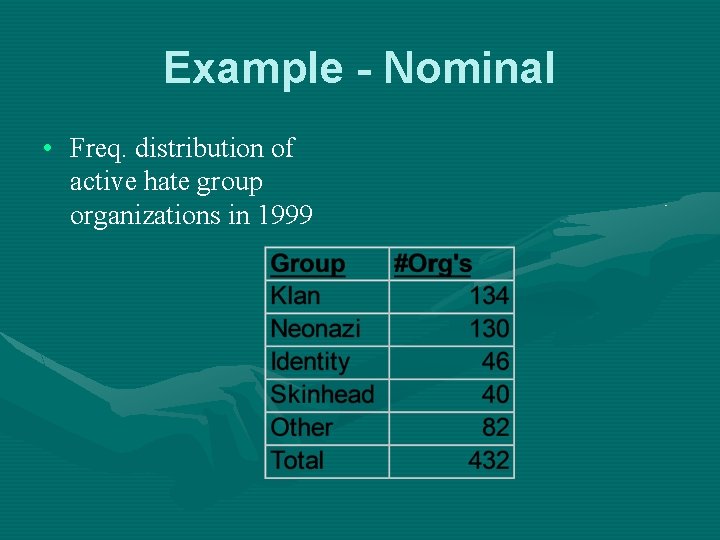
Example - Nominal • Freq. distribution of active hate group organizations in 1999

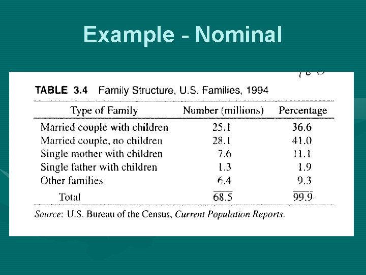
Example - Nominal

Summarizing Data in Graphs • Pie charts, Bar charts: appropriate for nominal variables and ordinal variables (small number of categories)

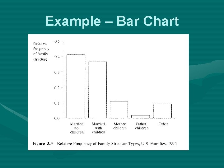
Example – Bar Chart

Summarizing Data in Graphs • Histograms: appropriate for all interval/ratio variables with a large number of possible values; data are collapsed into intervals, and axis labels represent interval boundaries or interval midpoints

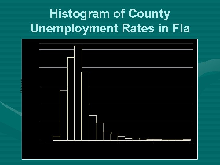
Histogram of County Unemployment Rates in Fla

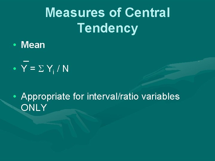
Measures of Central Tendency • Mean _ • Y = Yi / N • Appropriate for interval/ratio variables ONLY

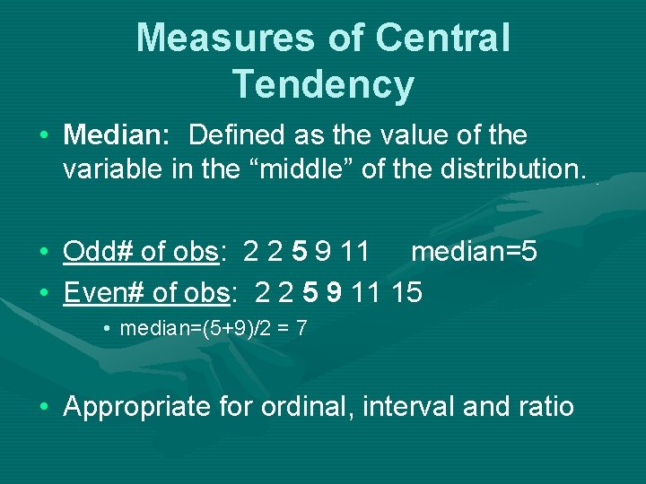
Measures of Central Tendency • Median: Defined as the value of the variable in the “middle” of the distribution. • Odd# of obs: 2 2 5 9 11 median=5 • Even# of obs: 2 2 5 9 11 15 • median=(5+9)/2 = 7 • Appropriate for ordinal, interval and ratio

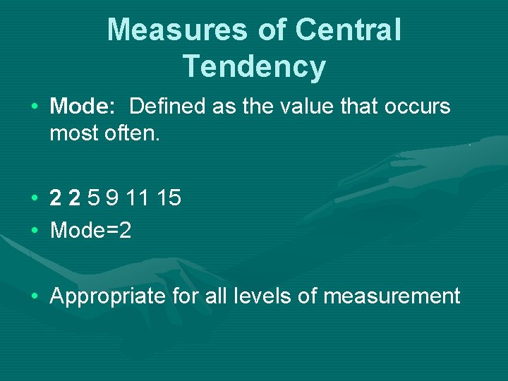
Measures of Central Tendency • Mode: Defined as the value that occurs most often. • 2 2 5 9 11 15 • Mode=2 • Appropriate for all levels of measurement

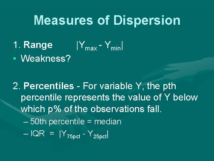
Measures of Dispersion 1. Range |Ymax - Ymin| • Weakness? 2. Percentiles - For variable Y, the pth percentile represents the value of Y below which p% of the observations fall. – 50 th percentile = median – IQR = |Y 75 pct - Y 25 pct|

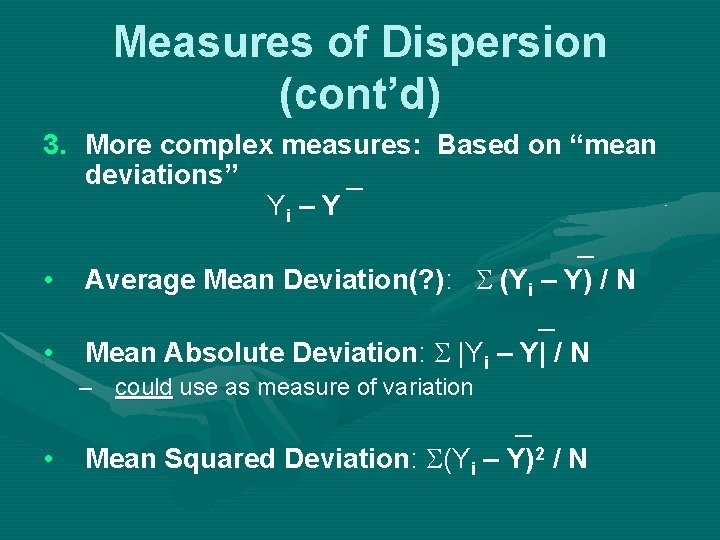
Measures of Dispersion (cont’d) 3. More complex measures: Based on “mean deviations” _ Yi – Y _ • Average Mean Deviation(? ): (Yi – Y) / N _ • Mean Absolute Deviation: |Yi – Y| / N – could use as measure of variation • _ Mean Squared Deviation: (Yi – Y)2 / N

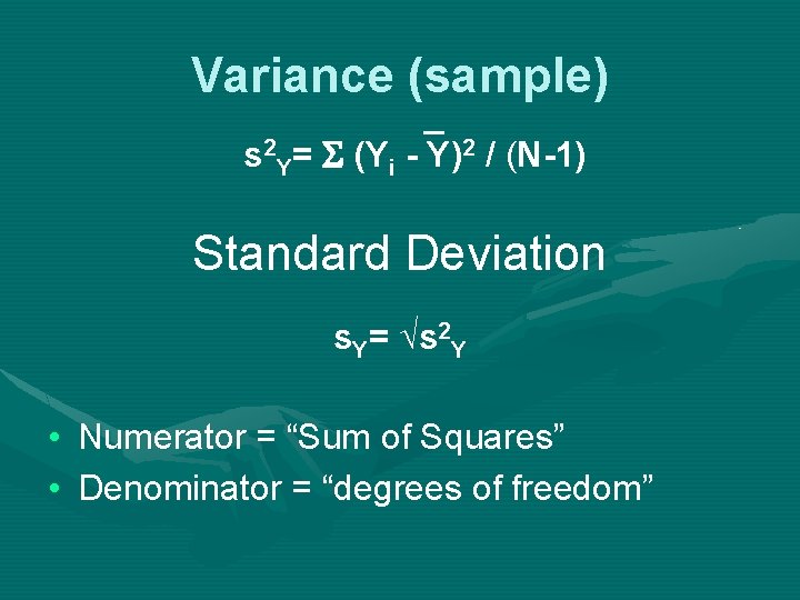
Variance (sample) _ s 2 Y= S (Yi - Y)2 / (N-1) Standard Deviation s. Y= √s 2 Y • Numerator = “Sum of Squares” • Denominator = “degrees of freedom”

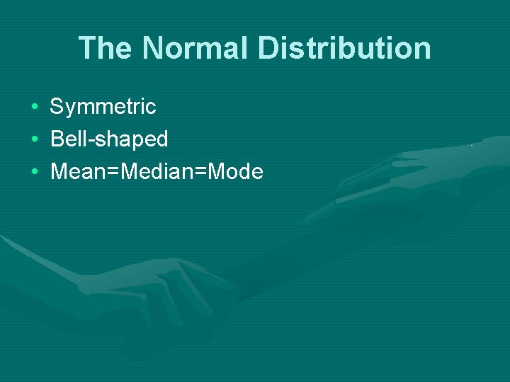
The Normal Distribution • • • Symmetric Bell-shaped Mean=Median=Mode

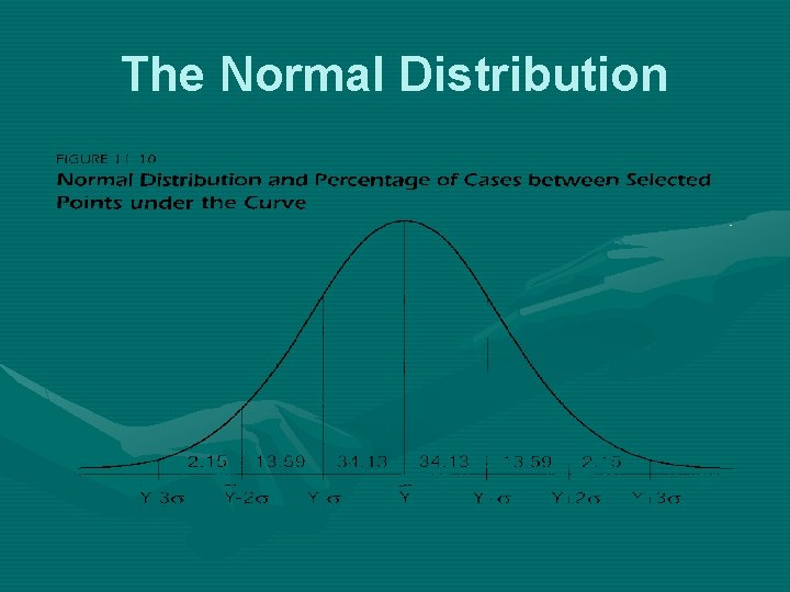
The Normal Distribution

Deviations from the normal distribution • Bimodal distributions • Skewed distributions – Left skew vs. right skew – Mean is pulled in direction of skew

Histogram of County Unemployment Rates in Fla

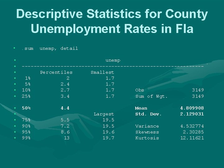
Descriptive Statistics for County Unemployment Rates in Fla • . sum unemp, detail • unemp • ------------------------------ • Percentiles Smallest • 1% 2 1. 7 • 5% 2. 4 1. 7 • 10% 2. 7 1. 7 Obs 3149 • 25% 3. 4 1. 7 Sum of Wgt. 3149 • • • 50% 75% 90% 95% 99% 4. 4 5. 5 7. 2 8. 6 13 Largest 19. 5 19. 6 19. 7 Mean Std. Dev. 4. 809908 2. 129031 Variance Skewness Kurtosis 4. 532774 2. 30285 12. 11621

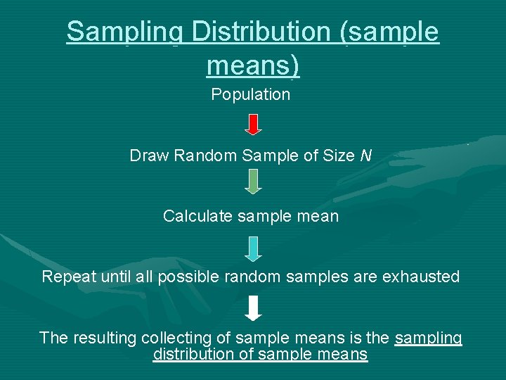
Sampling Distribution (sample means) Population Draw Random Sample of Size N Calculate sample mean Repeat until all possible random samples are exhausted The resulting collecting of sample means is the sampling distribution of sample means

Sampling Distribution of Sample Means • A frequency distribution of all possible sample means for a given sample size (N) • The mean of the sampling distribution will be equal to the population mean.

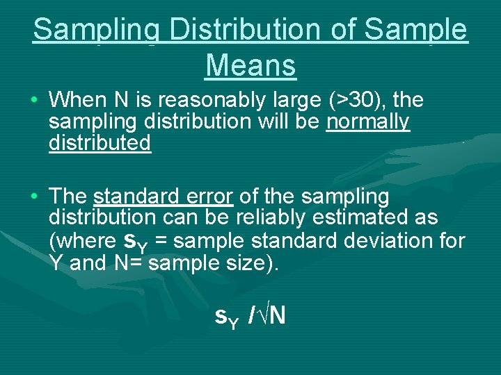
Sampling Distribution of Sample Means • When N is reasonably large (>30), the sampling distribution will be normally distributed • The standard error of the sampling distribution can be reliably estimated as (where s. Y = sample standard deviation for Y and N= sample size). s. Y /√N

Standard Error • How the sample means vary from sample to sample (i. e. within the sampling distribution) is expressed statistically by the value of the standard deviation (i. e. standard error) of the sampling distribution. • (Standard deviation = the “average” distance of each observation from the mean)

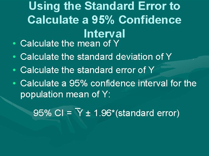
• • Using the Standard Error to Calculate a 95% Confidence Interval Calculate the mean of Y Calculate the standard deviation of Y Calculate the standard error of Y Calculate a 95% confidence interval for the population mean of Y: _ 95% CI = Y ± 1. 96*(standard error)

Example • Hillary Clinton Feeling Thermometer (NES 2004)

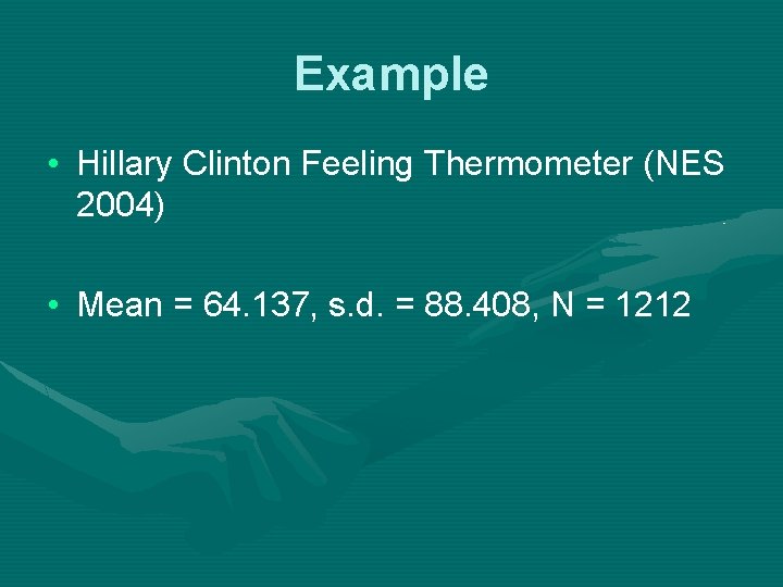
Example • Hillary Clinton Feeling Thermometer (NES 2004) • Mean = 64. 137, s. d. = 88. 408, N = 1212

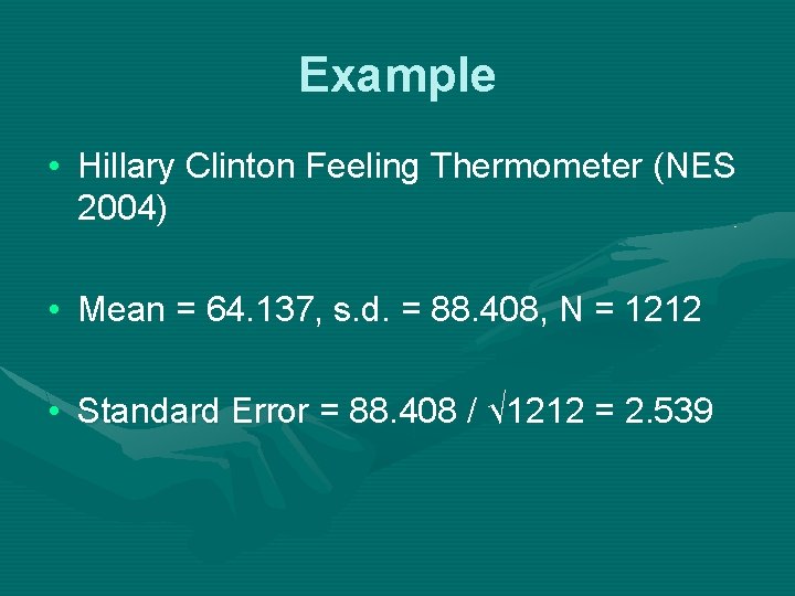
Example • Hillary Clinton Feeling Thermometer (NES 2004) • Mean = 64. 137, s. d. = 88. 408, N = 1212 • Standard Error = 88. 408 / √ 1212 = 2. 539

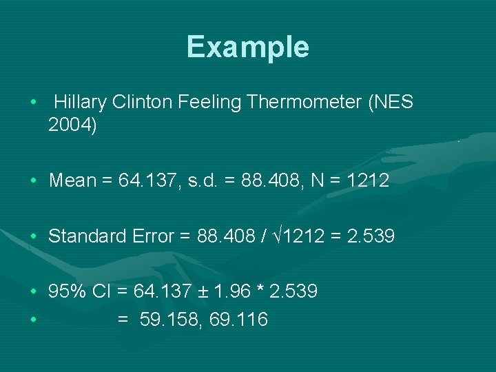
Example • Hillary Clinton Feeling Thermometer (NES 2004) • Mean = 64. 137, s. d. = 88. 408, N = 1212 • Standard Error = 88. 408 / √ 1212 = 2. 539 • 95% CI = 64. 137 ± 1. 96 * 2. 539 • = 59. 158, 69. 116