UNITI AMPLITUDE MODULATION M N Narsaiah Assoc professor

UNIT-I AMPLITUDE MODULATION M. N. Narsaiah, Assoc professor

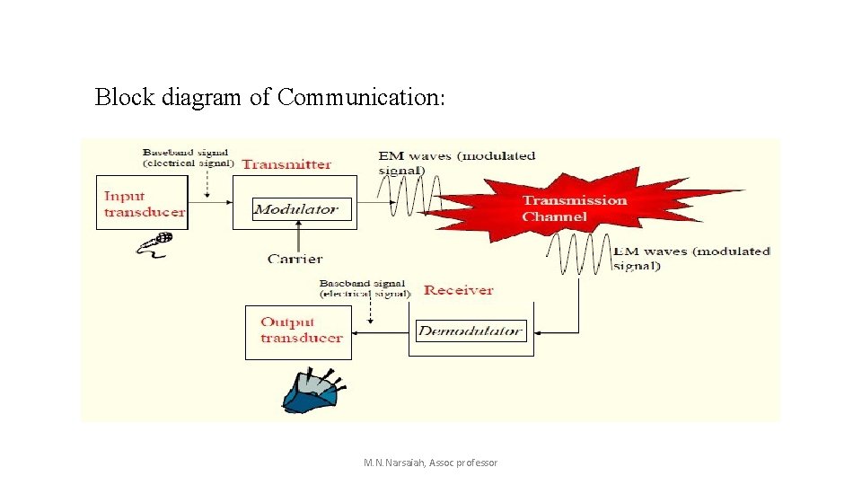
Communication Systems: • Communication deals with the principle of transferring information from one place to another. • The source could be in continuous form as in the case of analog communication and as discrete signals as in the case of digital communication. • Short distance transmission of information is called baseband transmission. • For long distance transmission, information has to be impressed upon an high frequency component to be able to reach the reception end of communication. • The high frequency component is termed as a carrier and the entire process is called modulation. M. N. Narsaiah, Assoc professor

Block diagram of Communication: M. N. Narsaiah, Assoc professor

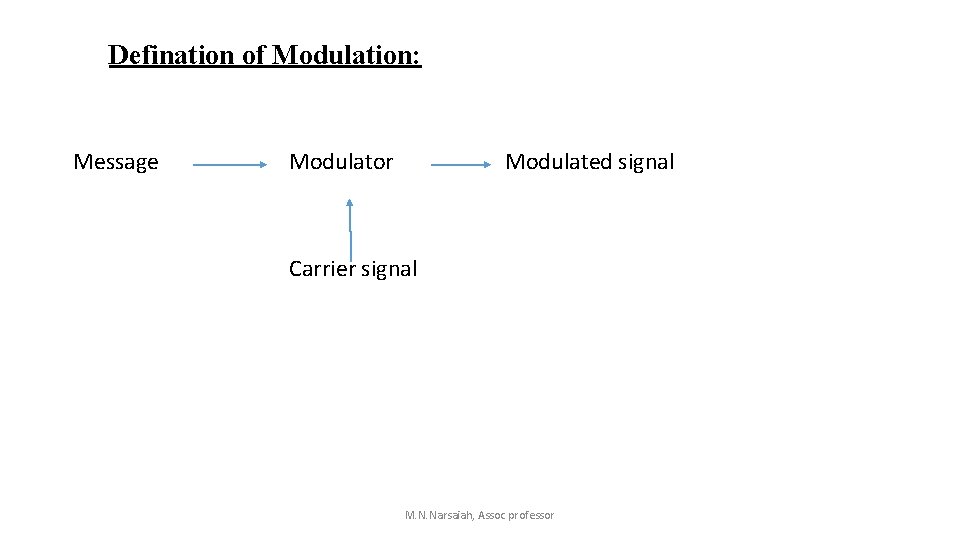
Defination of Modulation: Message Modulator Modulated signal Carrier signal M. N. Narsaiah, Assoc professor

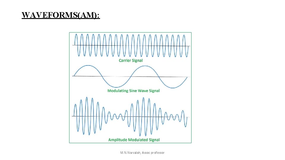
WAVEFORMS(AM): M. N. Narsaiah, Assoc professor

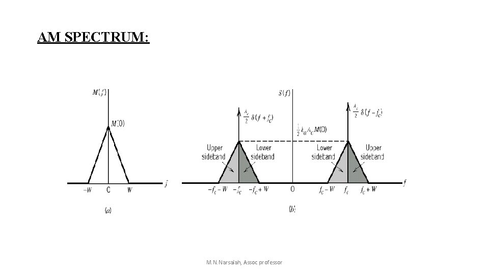
AM SPECTRUM: M. N. Narsaiah, Assoc professor

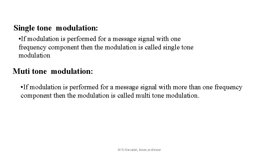
Single tone modulation: • If modulation is performed for a message signal with one frequency component then the modulation is called single tone modulation Muti tone modulation: • If modulation is performed for a message signal with more than one frequency component then the modulation is called multi tone modulation. M. N. Narsaiah, Assoc professor

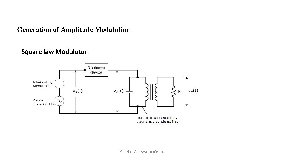
Generation of Amplitude Modulation: Square law Modulator: M. N. Narsaiah, Assoc professor

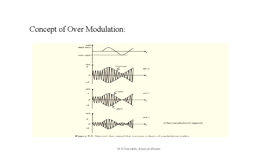
Concept of Over Modulation: M. N. Narsaiah, Assoc professor

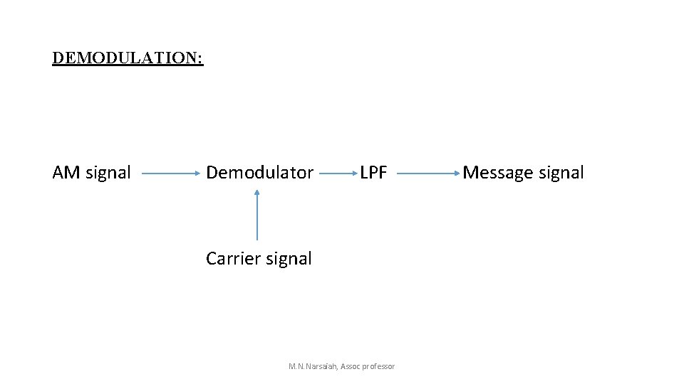
DEMODULATION: AM signal Demodulator LPF Carrier signal M. N. Narsaiah, Assoc professor Message signal

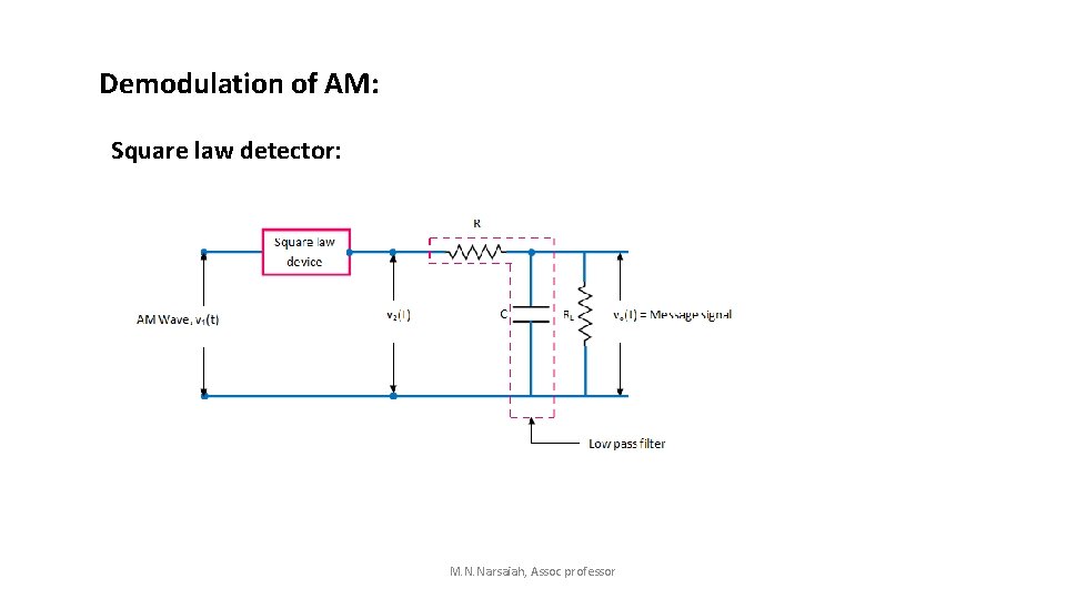
Demodulation of AM: Square law detector: M. N. Narsaiah, Assoc professor

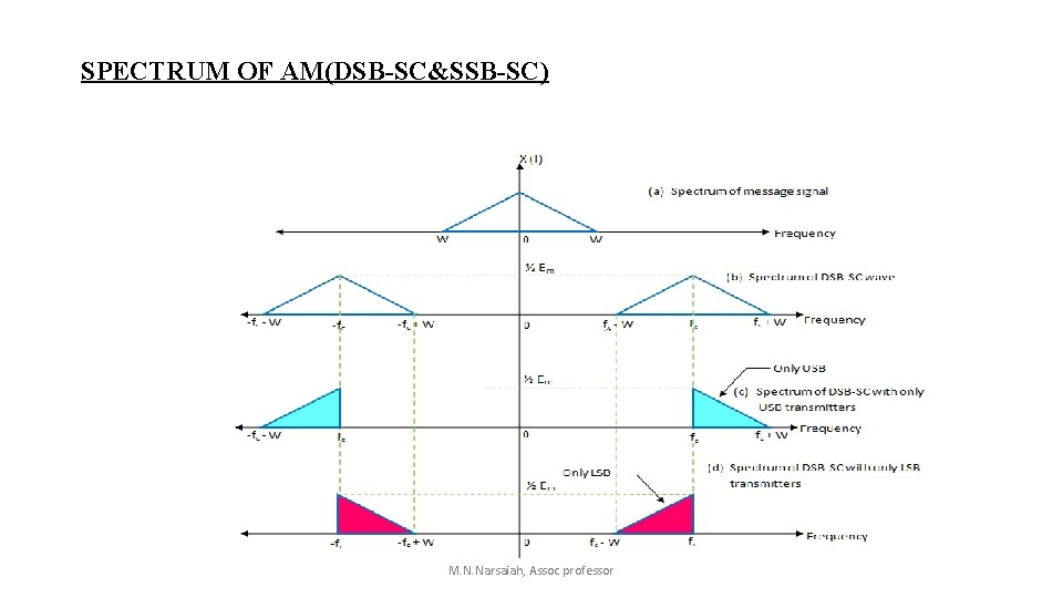
SPECTRUM OF AM(DSB-SC&SSB-SC) M. N. Narsaiah, Assoc professor

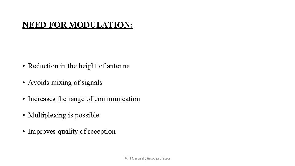
NEED FOR MODULATION: • Reduction in the height of antenna • Avoids mixing of signals • Increases the range of communication • Multiplexing is possible • Improves quality of reception M. N. Narsaiah, Assoc professor

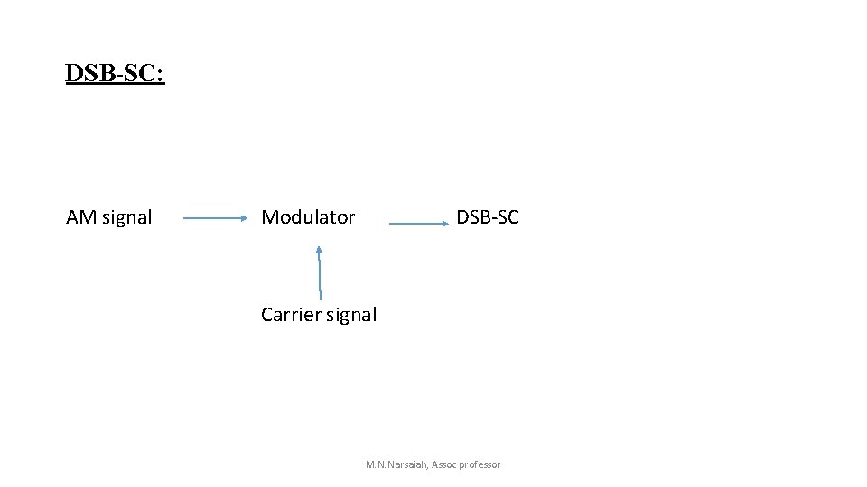
DSB-SC: AM signal Modulator DSB-SC Carrier signal M. N. Narsaiah, Assoc professor

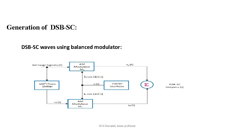
Generation of DSB-SC: DSB-SC waves using balanced modulator: M. N. Narsaiah, Assoc professor

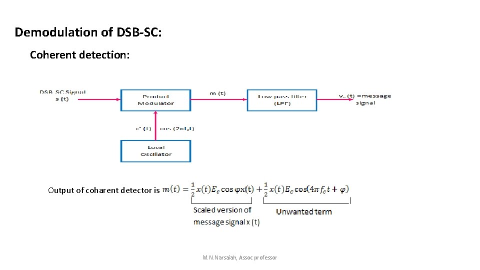
Demodulation of DSB-SC: Coherent detection: Output of coharent detector is M. N. Narsaiah, Assoc professor

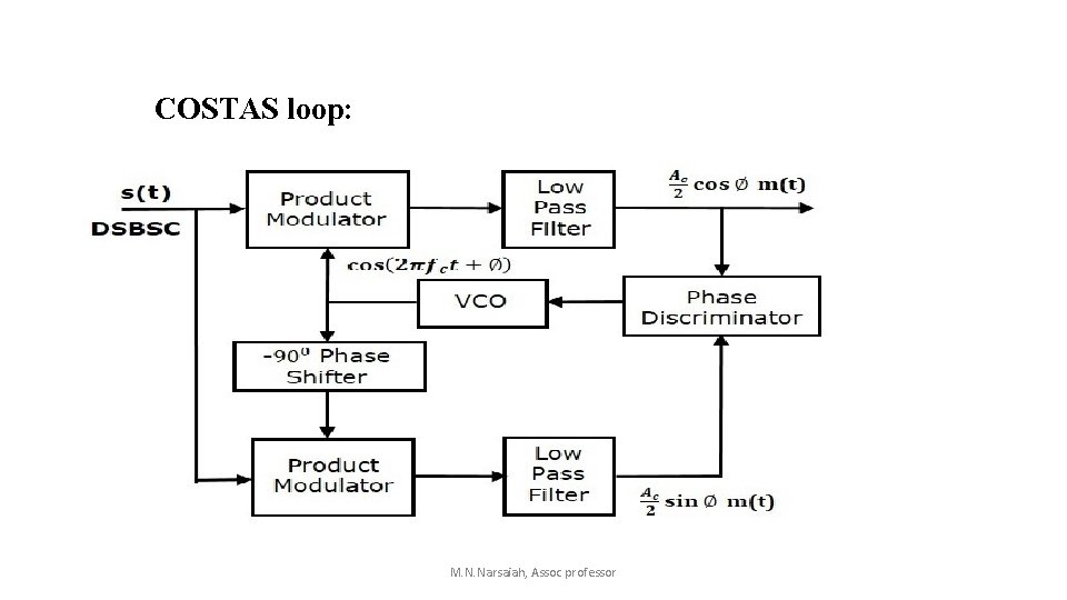
COSTAS loop: M. N. Narsaiah, Assoc professor

M. N. Narsaiah, Assoc professor

UNIT II SSB MODULATION M. N. Narsaiah, Assoc Professor

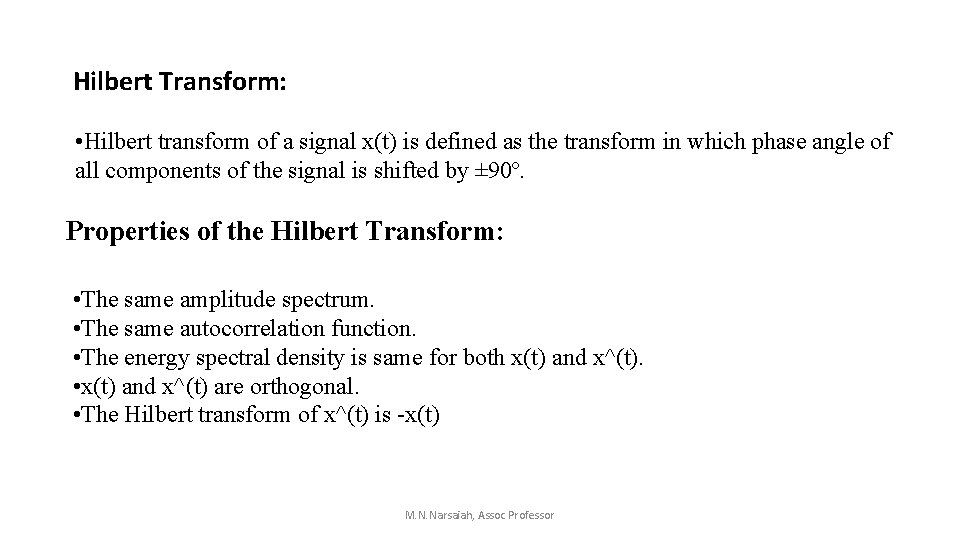
Hilbert Transform: • Hilbert transform of a signal x(t) is defined as the transform in which phase angle of all components of the signal is shifted by ± 90º. Properties of the Hilbert Transform: • The same amplitude spectrum. • The same autocorrelation function. • The energy spectral density is same for both x(t) and x^(t). • x(t) and x^(t) are orthogonal. • The Hilbert transform of x^(t) is -x(t) M. N. Narsaiah, Assoc Professor

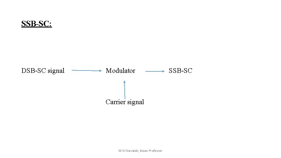
SSB-SC: DSB-SC signal Modulator Carrier signal M. N. Narsaiah, Assoc Professor SSB-SC

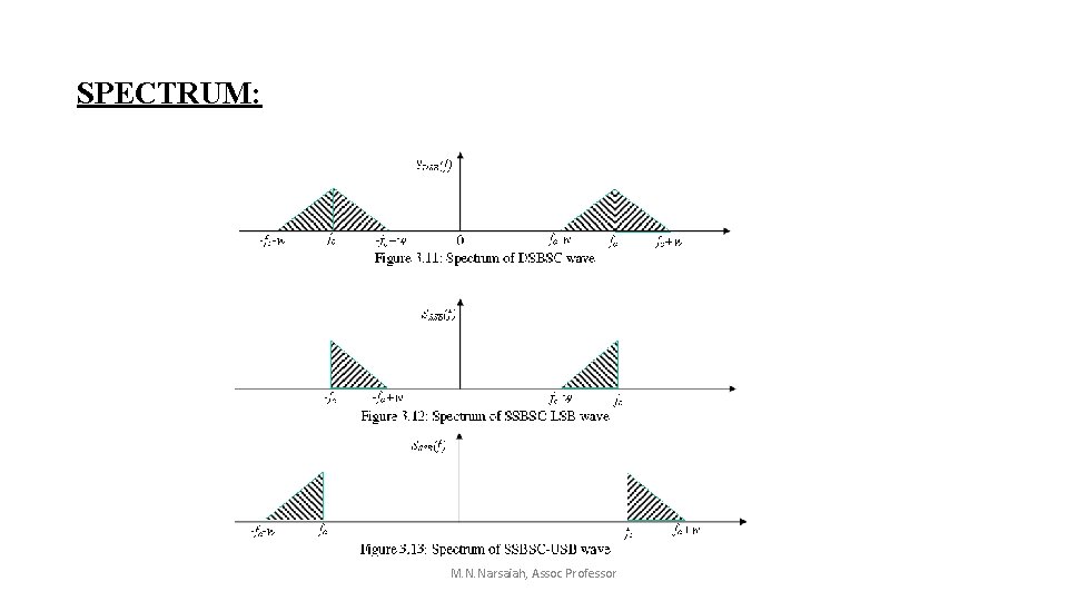
SPECTRUM: M. N. Narsaiah, Assoc Professor

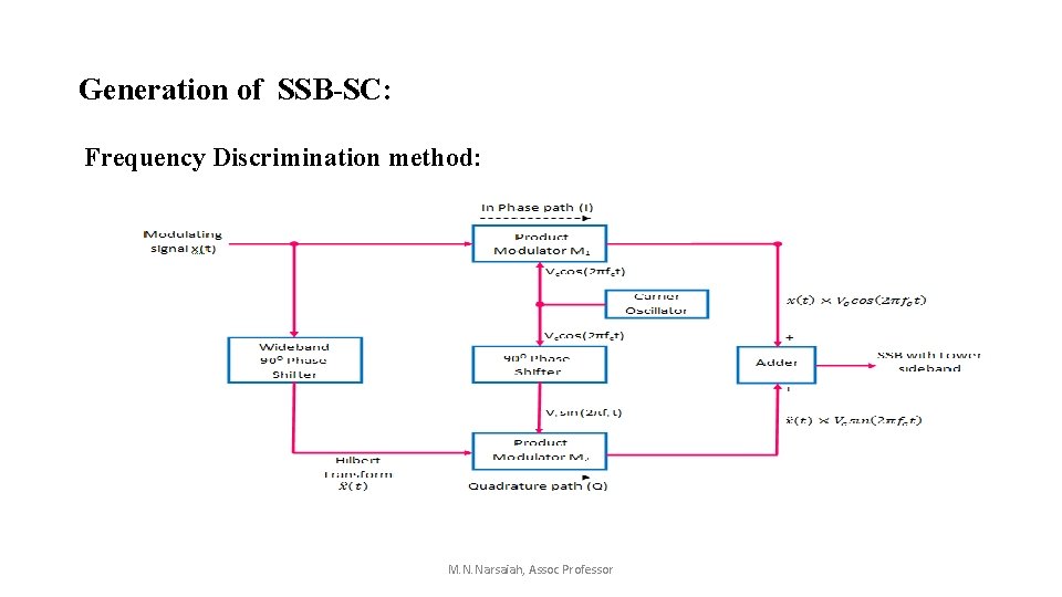
Generation of SSB-SC: Frequency Discrimination method: M. N. Narsaiah, Assoc Professor

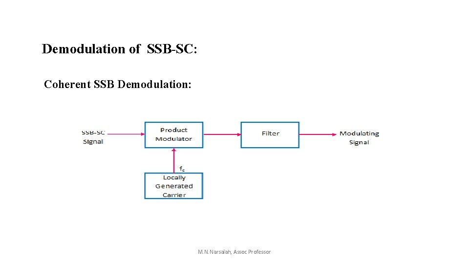
Demodulation of SSB-SC: Coherent SSB Demodulation: M. N. Narsaiah, Assoc Professor

ADVANTAGES • Lower power consumption • Better management of the frequency spectrum • Less prone to selective fading • Lower noise M. N. Narsaiah, Assoc Professor

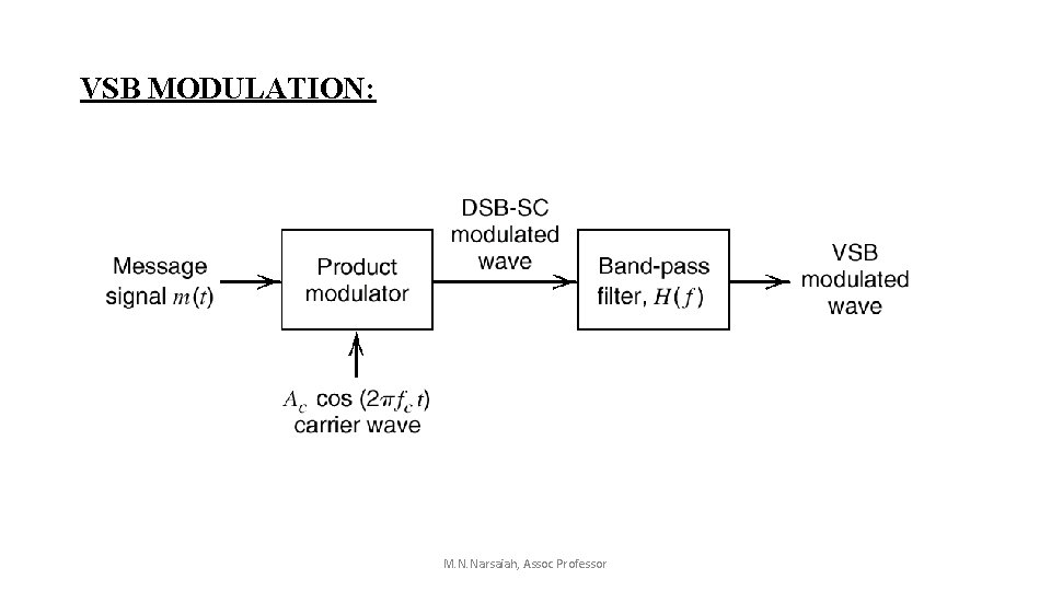
VSB MODULATION: M. N. Narsaiah, Assoc Professor

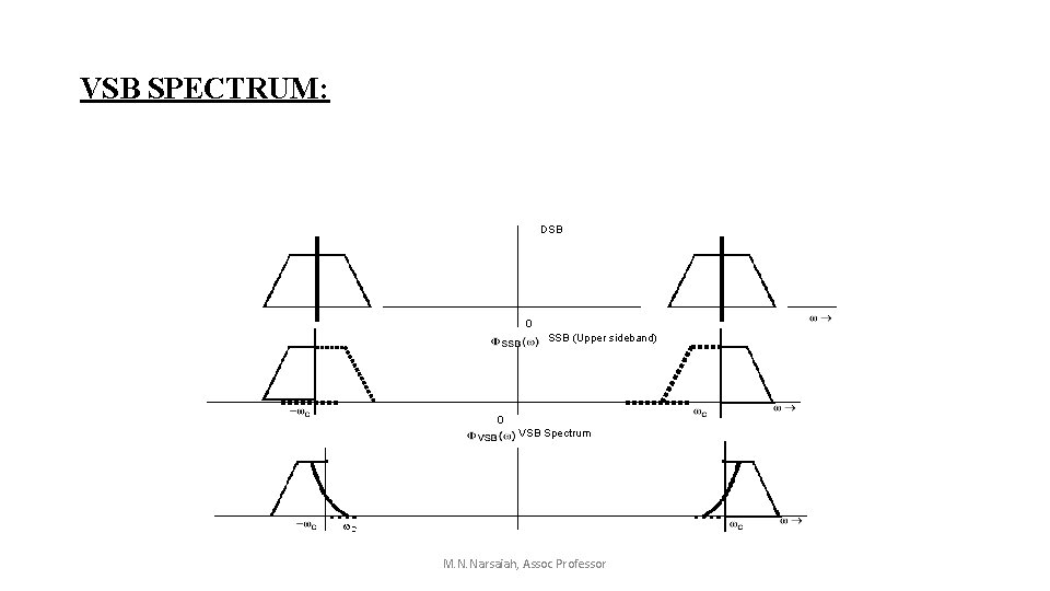
VSB SPECTRUM: DSB 0 SSB (Upper sideband) 0 VSB Spectrum M. N. Narsaiah, Assoc Professor

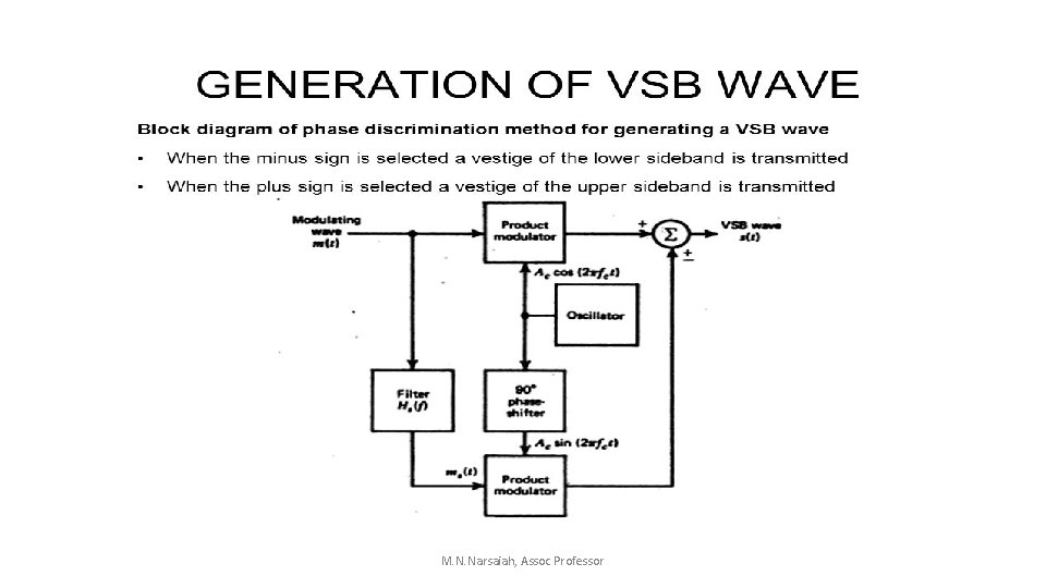
M. N. Narsaiah, Assoc Professor

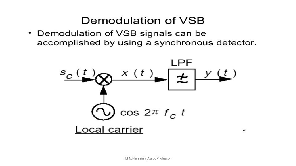
M. N. Narsaiah, Assoc Professor

ADVANTAGES: • The main advantage of VSB modulation is the reduction in bandwidth. It is almost as efficient as the SSB. • Due to allowance of transmitting a part of lower sideband, the constraint on the filter have been relaxed So practically, easy to design filters can be used. • It possesses good phase characteristics and makes the transmission of low frequency components possible. M. N. Narsaiah, Assoc Professor

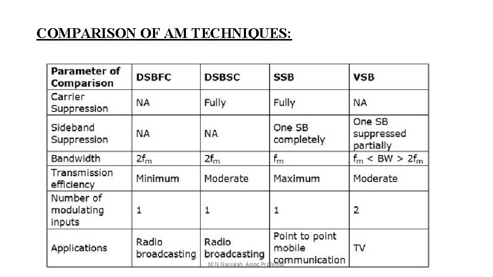
COMPARISON OF AM TECHNIQUES: M. N. Narsaiah, Assoc Professor

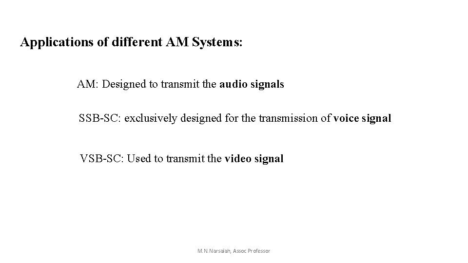
Applications of different AM Systems: AM: Designed to transmit the audio signals SSB-SC: exclusively designed for the transmission of voice signal VSB-SC: Used to transmit the video signal M. N. Narsaiah, Assoc Professor

M. N. Narsaiah, Assoc Professor

UNIT III ANGLE MODULATION M. N. Narsaiah, Assoc Professor

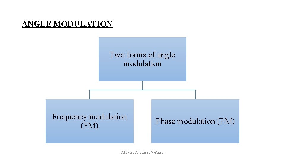
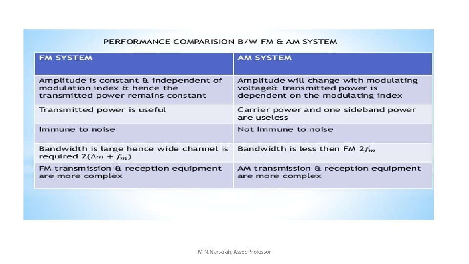
ANGLE MODULATION Two forms of angle modulation Frequency modulation (FM) Phase modulation (PM) M. N. Narsaiah, Assoc Professor

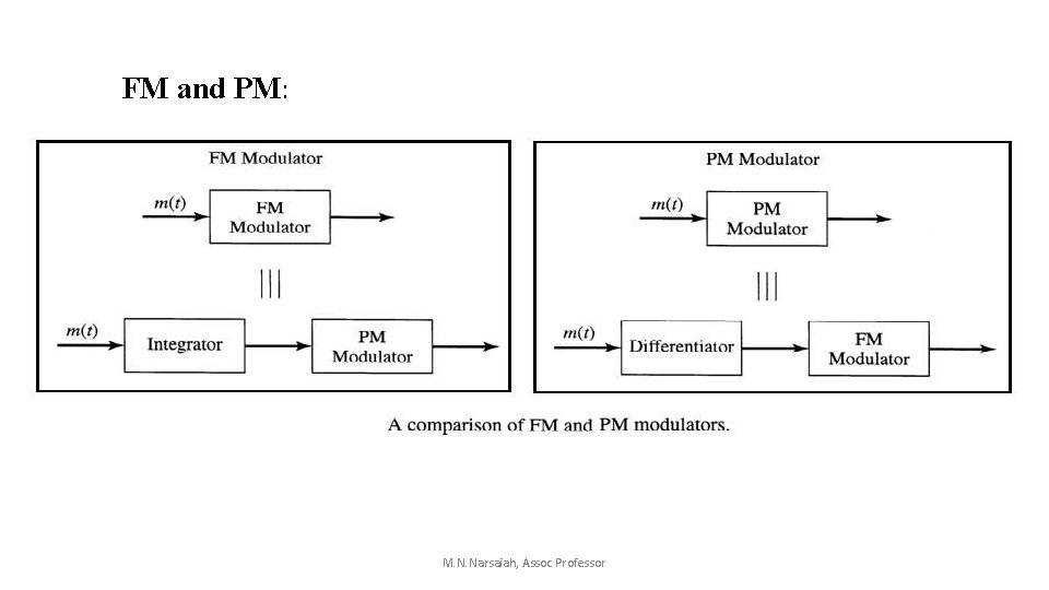
FM and PM: M. N. Narsaiah, Assoc Professor

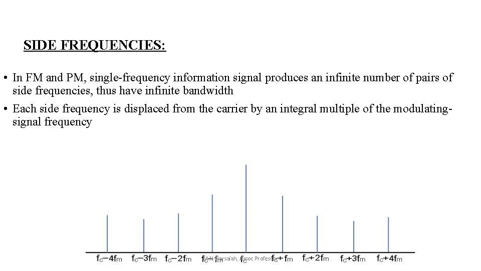
SIDE FREQUENCIES: • In FM and PM, single-frequency information signal produces an infinite number of pairs of side frequencies, thus have infinite bandwidth • Each side frequency is displaced from the carrier by an integral multiple of the modulatingsignal frequency M. N. Narsaiah, Assoc Professor

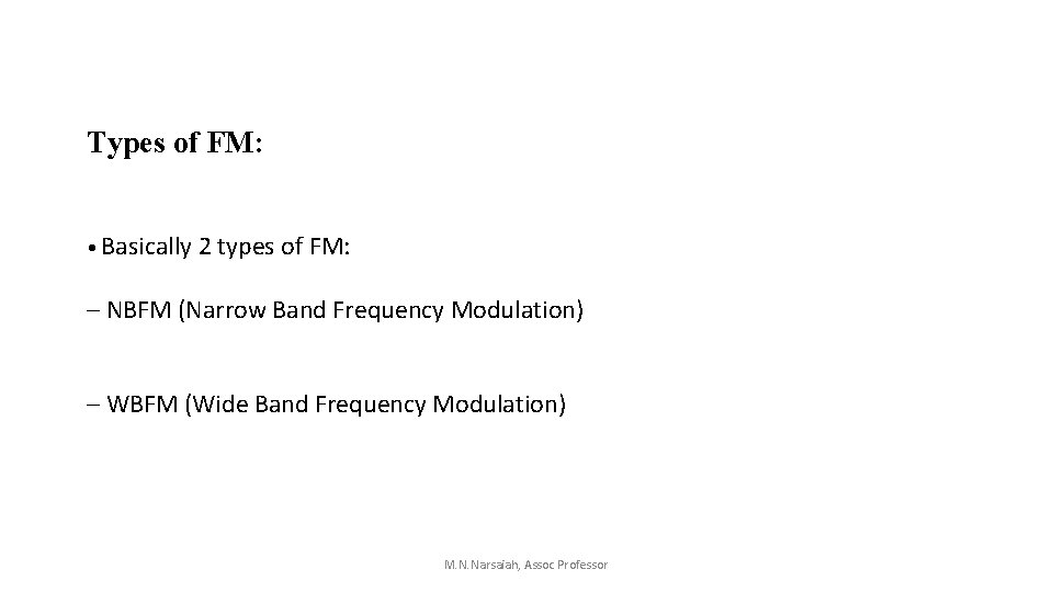
Types of FM: • Basically 2 types of FM: – NBFM (Narrow Band Frequency Modulation) – WBFM (Wide Band Frequency Modulation) M. N. Narsaiah, Assoc Professor

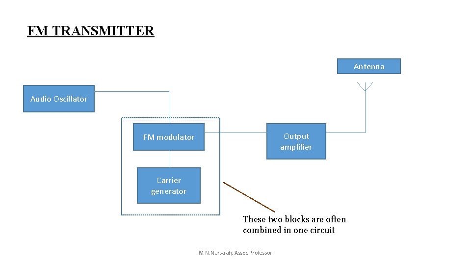
FM TRANSMITTER Antenna Audio Oscillator Output amplifier FM modulator Carrier generator These two blocks are often combined in one circuit M. N. Narsaiah, Assoc Professor

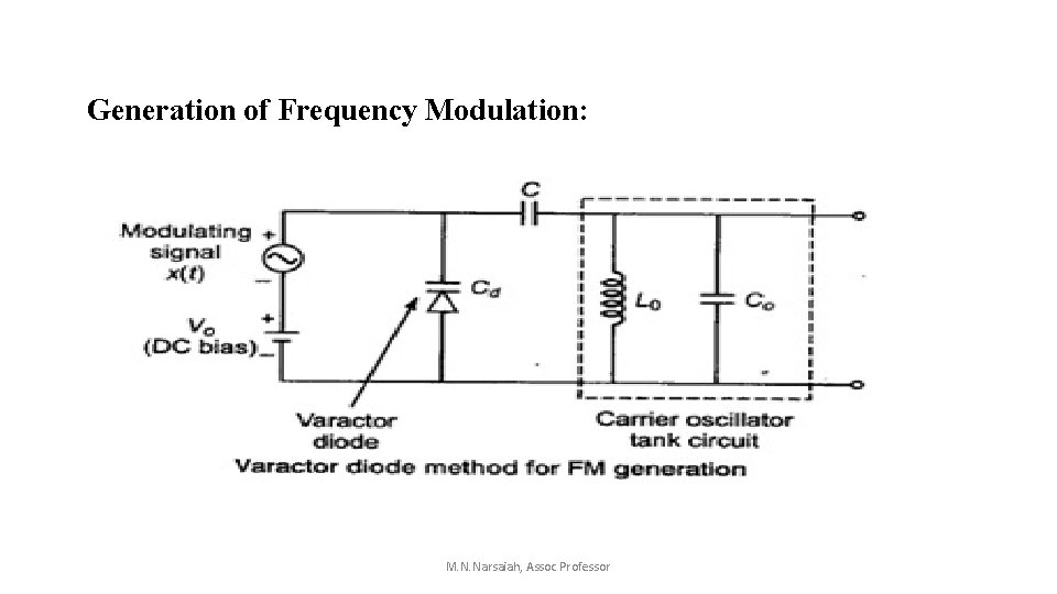
Generation of Frequency Modulation: M. N. Narsaiah, Assoc Professor

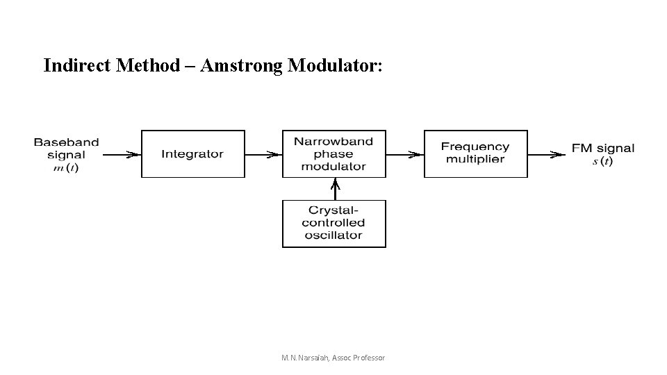
Indirect Method – Amstrong Modulator: M. N. Narsaiah, Assoc Professor

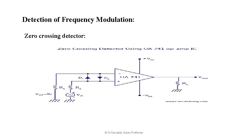
Detection of Frequency Modulation: Zero crossing detector: M. N. Narsaiah, Assoc Professor

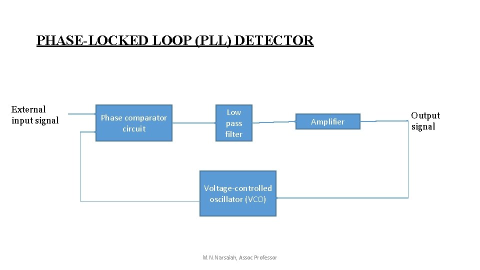
PHASE-LOCKED LOOP (PLL) DETECTOR External input signal Phase comparator circuit Low pass filter Voltage-controlled oscillator (VCO) M. N. Narsaiah, Assoc Professor Amplifier Output signal

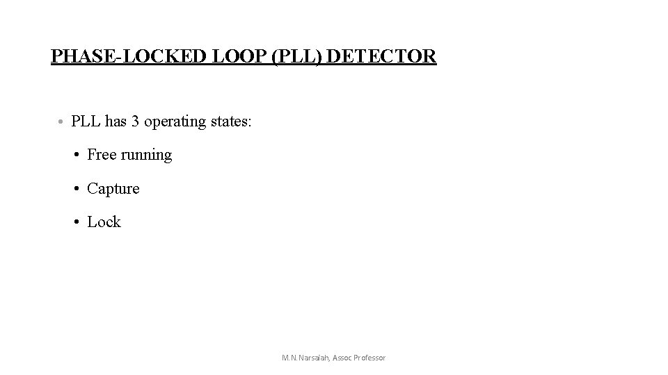
PHASE-LOCKED LOOP (PLL) DETECTOR • PLL has 3 operating states: • Free running • Capture • Lock M. N. Narsaiah, Assoc Professor

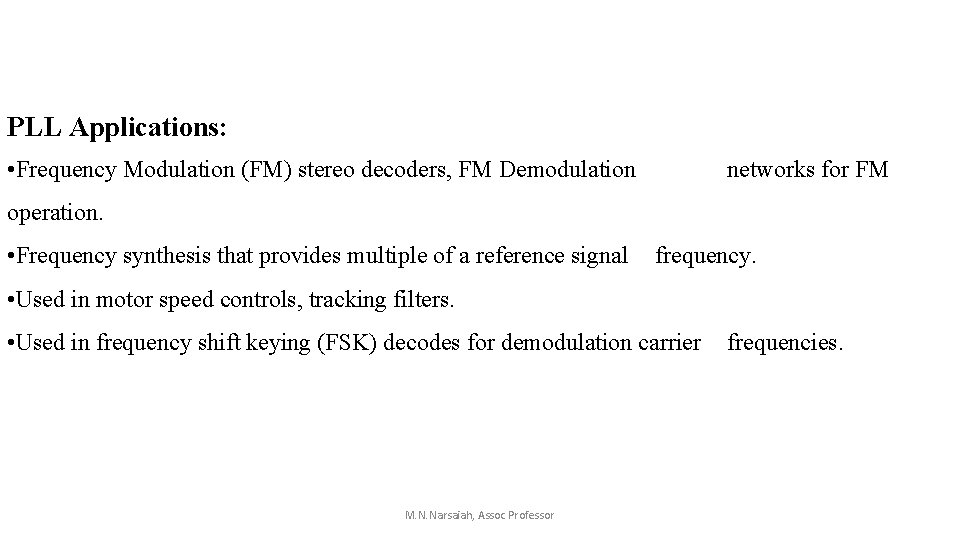
PLL Applications: • Frequency Modulation (FM) stereo decoders, FM Demodulation networks for FM operation. • Frequency synthesis that provides multiple of a reference signal frequency. • Used in motor speed controls, tracking filters. • Used in frequency shift keying (FSK) decodes for demodulation carrier frequencies. M. N. Narsaiah, Assoc Professor

APPLICATIONS OF ANGLE MODULATION • • • Radio Broadcasting Two way mobile radio Microwave communication TV sound transmission Cellular radio Satellite communication M. N. Narsaiah, Assoc Professor

M. N. Narsaiah, Assoc Professor

M. N. Narsaiah, Assoc Professor

Digital communications Introduction to digital communications

Introduction • digital communication is a mode of communication where the information or the thought is encoded digitally as discreet signals and electronically transferred to the recipients. • n digital communication information flows in a digital form and the source is generally the keyboard of the computer. A single individual is capable of digital communication and thus it also saves wastage of manpower and is one of the cheapest modes of communication. • Digital communication is also a really quick way to communicate. The information can reach the recipient within a fraction of a second. An individual no longer has to wait to personally meet the other individual and share his information.

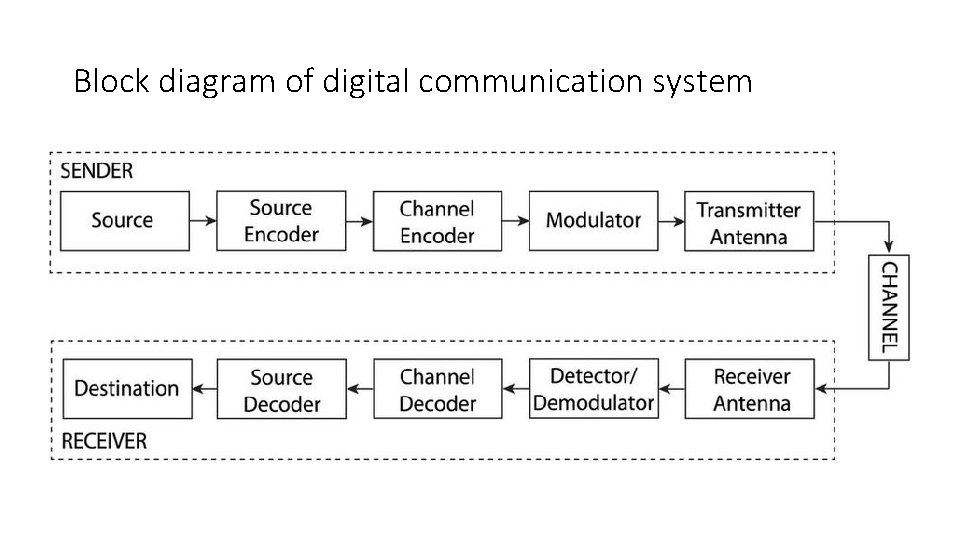
Block diagram of digital communication system

Advantages • The digital communication has mostly common structure of encoding a signal so devices used are mostly similar. • The Digital Communication's main advantage is that it provides us added security to our information signal. • The digital Communication system has more immunity to noise and external interference. • Digital information can be saved and retrieved when necessary while it is not possible in analog. • Digital Communication is cheaper than Analog Communication. • The configuring process of digital communication system is simple as compared to analog communication system. Although, they are complex. • In Digital Communication System, the error correction and detection techniques can be implemented easily.

Disadvantages • Disadvantages of digital communication: 1). Generally, more bandwidth is required than that for analog systems. 2). Synchronization is required. 3). High power consumption (Due to various stages of conversion). 4). Complex circuit, more sophisticated device making is also drawbacks of digital system. 5). Introduce sampling error 6). As square wave is more affected by noise, That’s why while communicating through channel we send sin waves but while operating on device we use squire pulses.

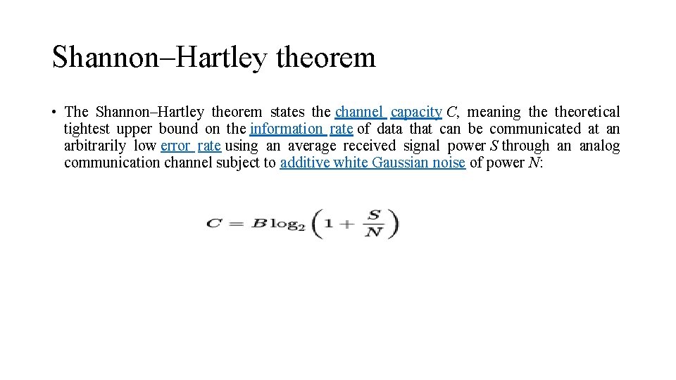
Shannon–Hartley theorem • The Shannon–Hartley theorem states the channel capacity C, meaning theoretical tightest upper bound on the information rate of data that can be communicated at an arbitrarily low error rate using an average received signal power S through an analog communication channel subject to additive white Gaussian noise of power N:

• Where C is the channel capacity in bits per second, a theoretical upper bound on the net bit rate (information rate, sometimes denoted I) excluding errorcorrection codes; • B is the bandwidth of the channel in hertz (passbandwidth in case of a bandpass signal); • S is the average received signal power over the bandwidth (in case of a carriermodulated passband transmission, often denoted C), measured in watts (or volts squared); • N is the average power of the noise and interference over the bandwidth, measured in watts (or volts squared); and • S/N is the signal-to-noise ratio (SNR) or the carrier-to-noise ratio (CNR) of the communication signal to the noise and interference at the receiver (expressed as a linear power ratio, not as logarithmic decibels).

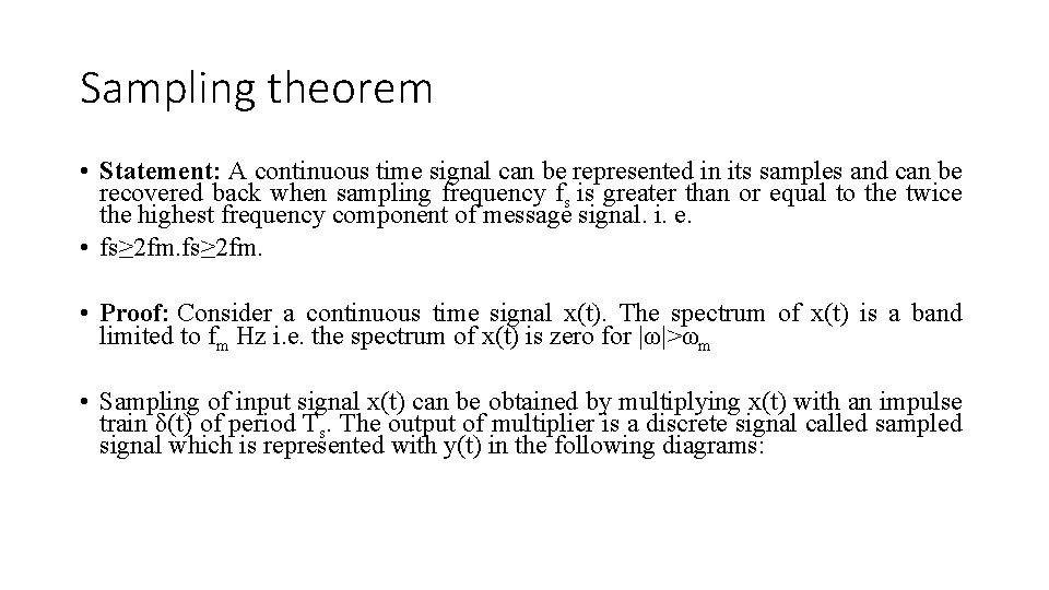
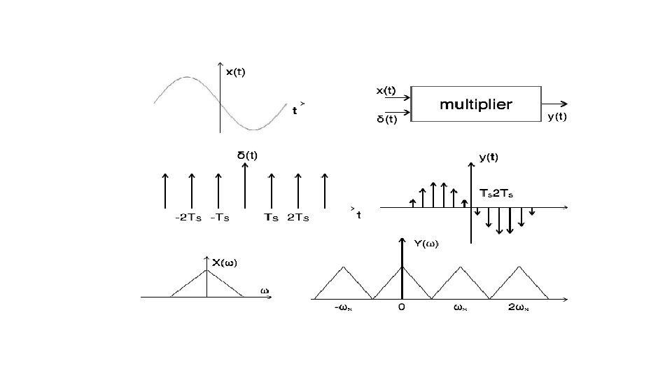
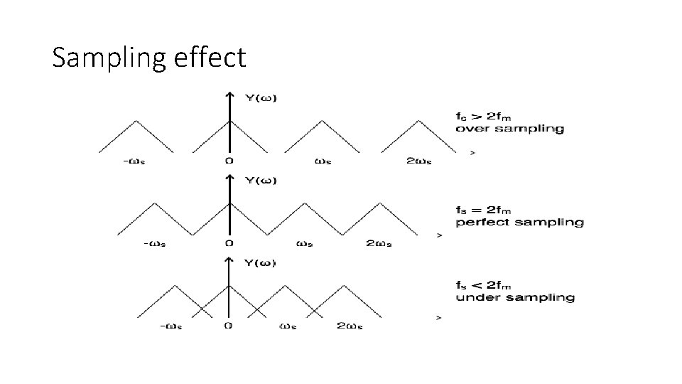
Sampling theorem • Statement: A continuous time signal can be represented in its samples and can be recovered back when sampling frequency fs is greater than or equal to the twice the highest frequency component of message signal. i. e. • fs≥ 2 fm. • Proof: Consider a continuous time signal x(t). The spectrum of x(t) is a band limited to fm Hz i. e. the spectrum of x(t) is zero for |ω|>ωm • Sampling of input signal x(t) can be obtained by multiplying x(t) with an impulse train δ(t) of period Ts. The output of multiplier is a discrete signal called sampled signal which is represented with y(t) in the following diagrams:

Sampling effect

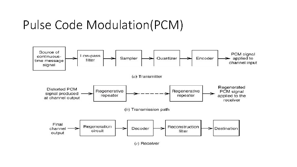
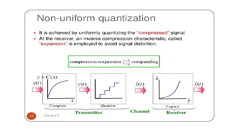
Pulse Code Modulation(PCM)

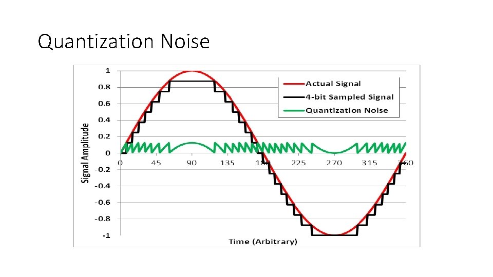
Quantization Noise

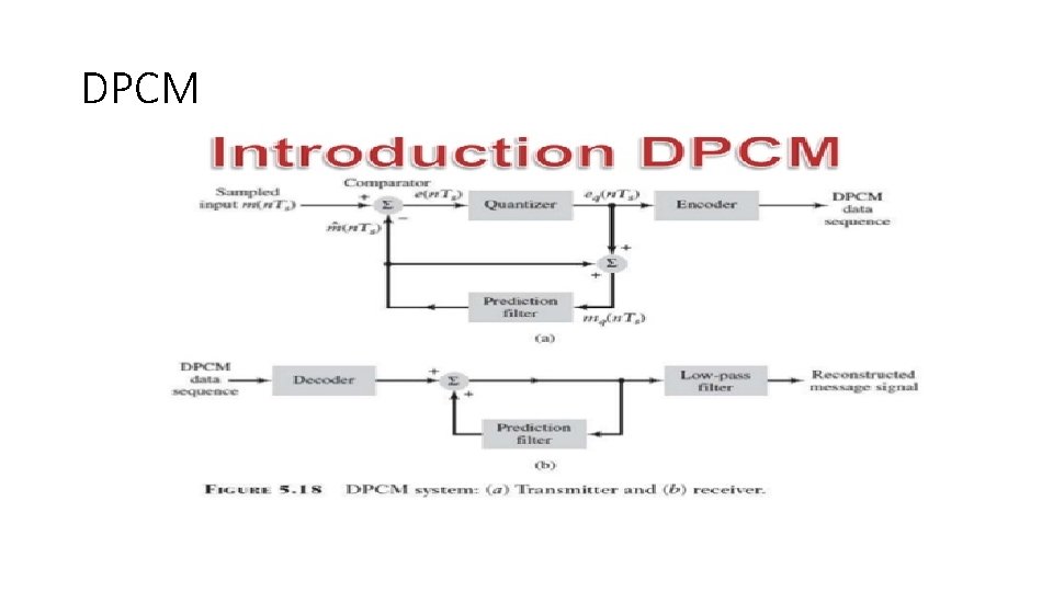
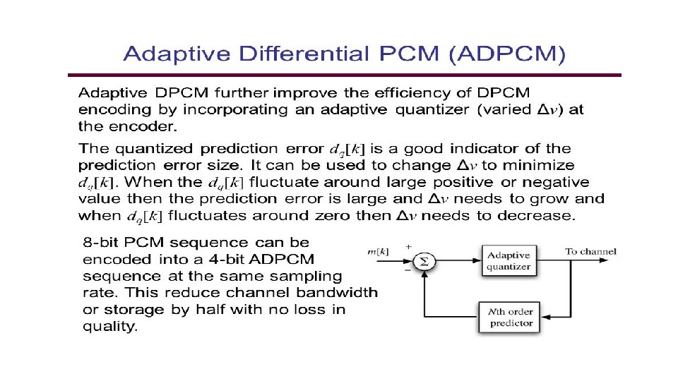
DPCM

Thank You!!!!

Error Control Codes Unit II

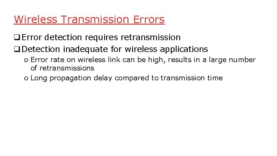
Wireless Transmission Errors q Error detection requires retransmission q Detection inadequate for wireless applications o Error rate on wireless link can be high, results in a large number of retransmissions o Long propagation delay compared to transmission time

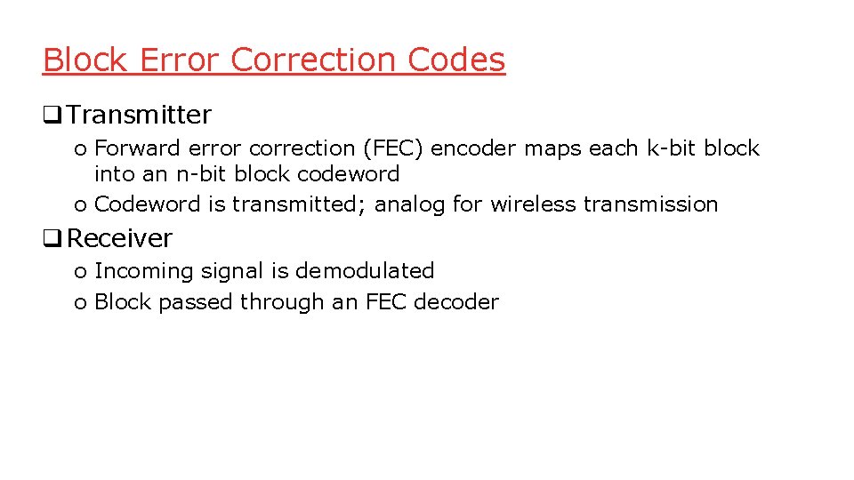
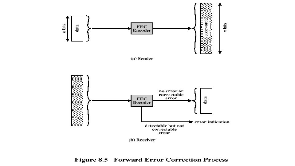
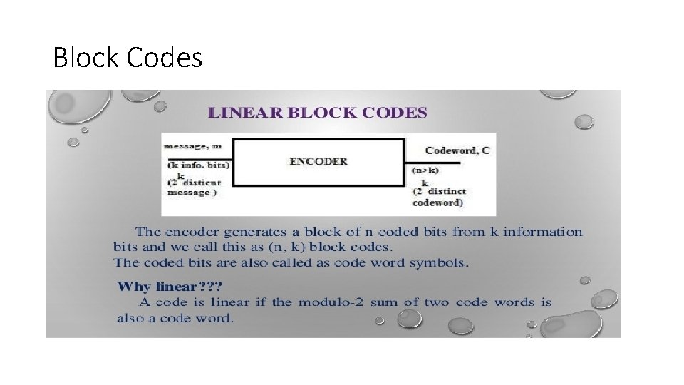
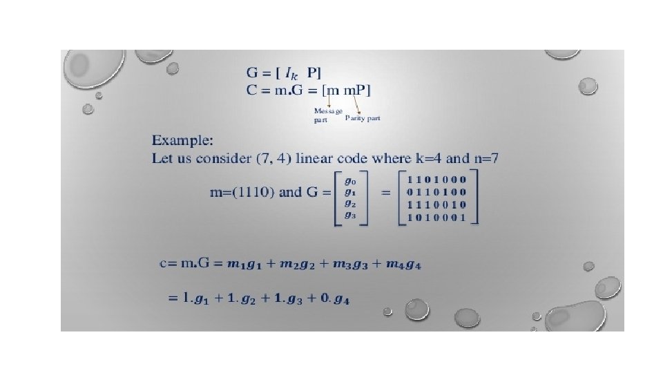
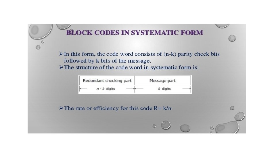
Block Error Correction Codes q Transmitter o Forward error correction (FEC) encoder maps each k-bit block into an n-bit block codeword o Codeword is transmitted; analog for wireless transmission q Receiver o Incoming signal is demodulated o Block passed through an FEC decoder

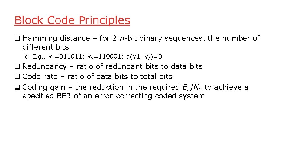
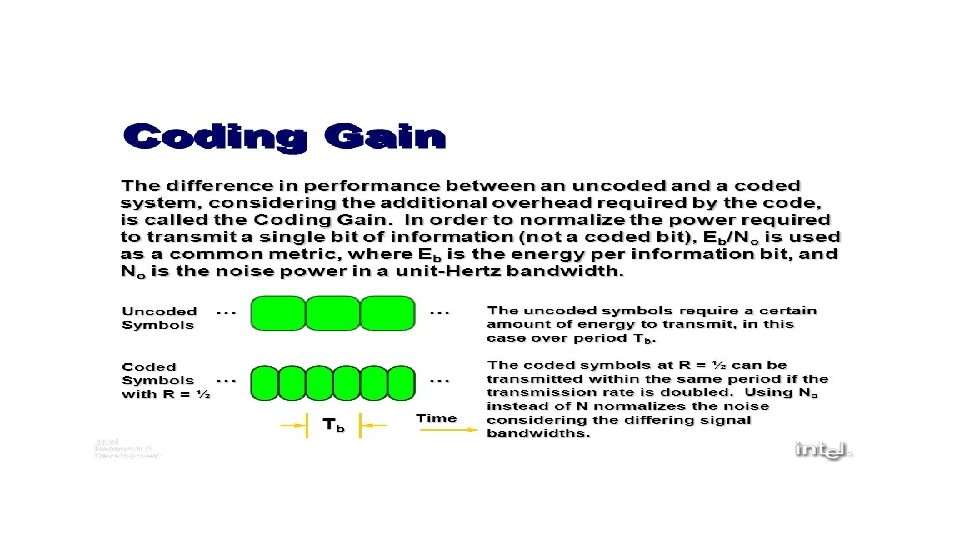
Block Code Principles q Hamming distance – for 2 n-bit binary sequences, the number of different bits o E. g. , v 1=011011; v 2=110001; d(v 1, v 2)=3 q Redundancy – ratio of redundant bits to data bits q Code rate – ratio of data bits to total bits q Coding gain – the reduction in the required Eb/N 0 to achieve a specified BER of an error-correcting coded system

Block Codes

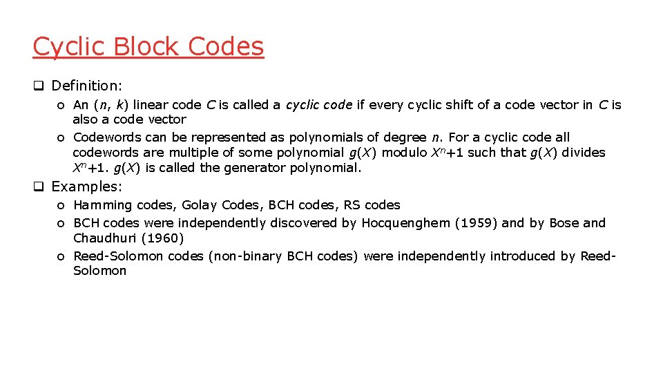
Cyclic Block Codes q Definition: o An (n, k) linear code C is called a cyclic code if every cyclic shift of a code vector in C is also a code vector o Codewords can be represented as polynomials of degree n. For a cyclic code all codewords are multiple of some polynomial g(X) modulo Xn+1 such that g(X) divides Xn+1. g(X) is called the generator polynomial. q Examples: o Hamming codes, Golay Codes, BCH codes, RS codes o BCH codes were independently discovered by Hocquenghem (1959) and by Bose and Chaudhuri (1960) o Reed-Solomon codes (non-binary BCH codes) were independently introduced by Reed. Solomon

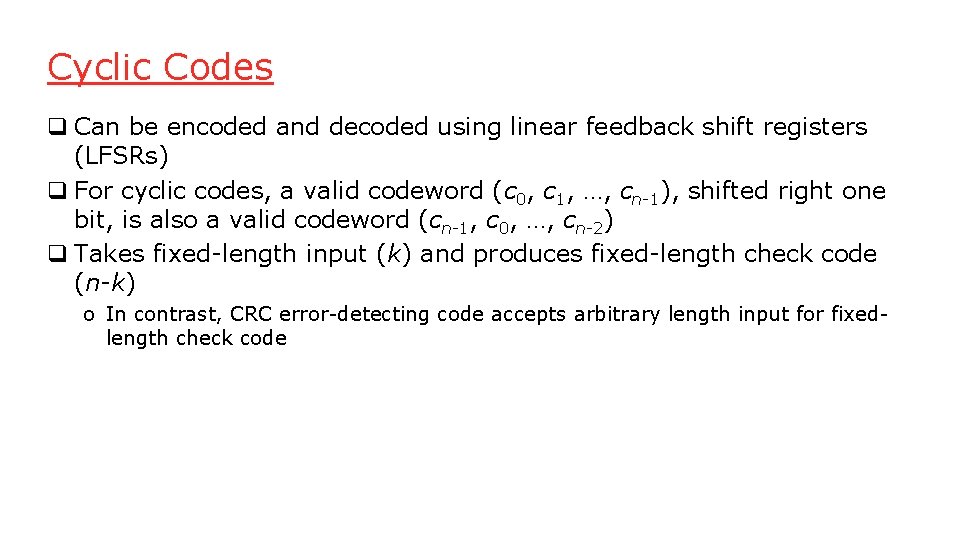
Cyclic Codes q Can be encoded and decoded using linear feedback shift registers (LFSRs) q For cyclic codes, a valid codeword (c 0, c 1, …, cn-1), shifted right one bit, is also a valid codeword (cn-1, c 0, …, cn-2) q Takes fixed-length input (k) and produces fixed-length check code (n-k) o In contrast, CRC error-detecting code accepts arbitrary length input for fixedlength check code

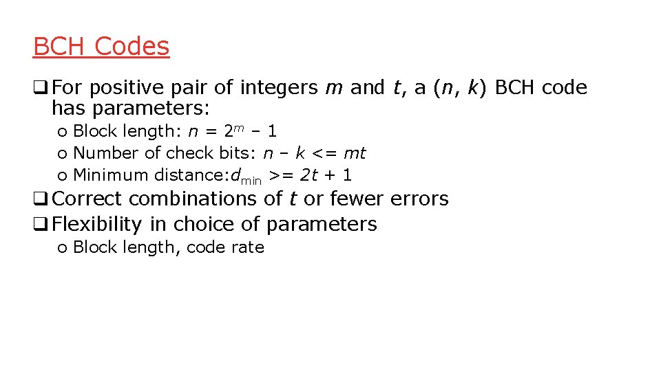
BCH Codes q For positive pair of integers m and t, a (n, k) BCH code has parameters: o Block length: n = 2 m – 1 o Number of check bits: n – k <= mt o Minimum distance: dmin >= 2 t + 1 q Correct combinations of t or fewer errors q Flexibility in choice of parameters o Block length, code rate

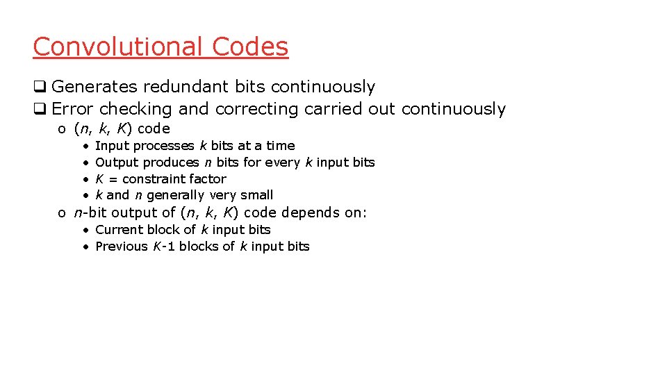
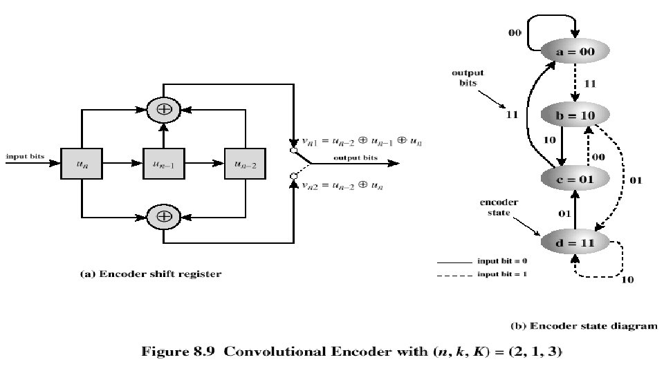
Convolutional Codes q Generates redundant bits continuously q Error checking and correcting carried out continuously o (n, k, K) code • • Input processes k bits at a time Output produces n bits for every k input bits K = constraint factor k and n generally very small o n-bit output of (n, k, K) code depends on: • Current block of k input bits • Previous K-1 blocks of k input bits

Convolutional Encoder

Decoding q Trellis diagram – expanded encoder diagram q Viterbi code – error correction algorithm o Compares received sequence with all possible transmitted sequences o Algorithm chooses path through trellis whose coded sequence differs from received sequence in the fewest number of places o Once a valid path is selected as the correct path, the decoder can recover the input data bits from the output code bits

Error Control q Mechanisms to detect and correct transmission errors q Types of errors: o Lost PDU : a PDU fails to arrive o Damaged PDU : PDU arrives with errors q Techniques: o Timeouts o Acknowledgments o Negative acknowledgments

Quotes about Shannon § ”What is information? Sidestepping questions about meaning, Shannon showed that it is a measurable commodity”. § ”Today, Shannon’s insight help shape virtually all systems that store, process, or transmit information in digital form, from compact discs to computers, from facsimile machines to deep space probes”. § ”Information theory has also infilitrated fields outside communications, including linguistics, psychology, economics, biology, even the arts”.

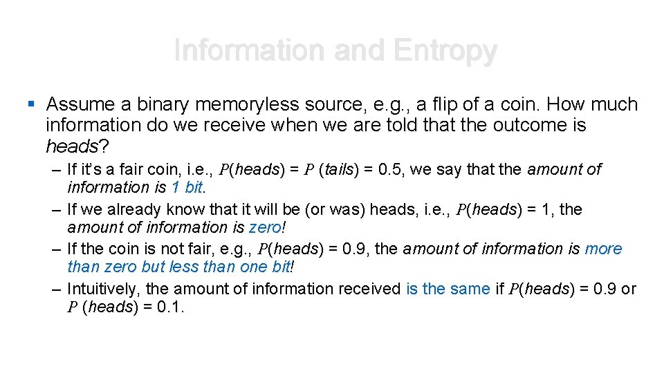
Information and Entropy § Assume a binary memoryless source, e. g. , a flip of a coin. How much information do we receive when we are told that the outcome is heads? – If it’s a fair coin, i. e. , P(heads) = P (tails) = 0. 5, we say that the amount of information is 1 bit. – If we already know that it will be (or was) heads, i. e. , P(heads) = 1, the amount of information is zero! – If the coin is not fair, e. g. , P(heads) = 0. 9, the amount of information is more than zero but less than one bit! – Intuitively, the amount of information received is the same if P(heads) = 0. 9 or P (heads) = 0. 1.

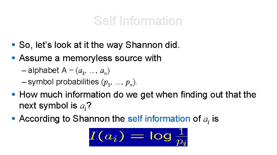
Self Information § So, let’s look at it the way Shannon did. § Assume a memoryless source with – alphabet A = (a 1, …, an) – symbol probabilities (p 1, …, pn). § How much information do we get when finding out that the next symbol is ai? § According to Shannon the self information of ai is

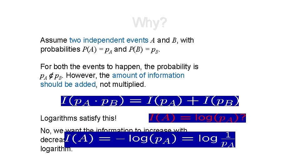
Why? Assume two independent events A and B, with probabilities P(A) = p. A and P(B) = p. B. For both the events to happen, the probability is p. A ¢ p. B. However, the amount of information should be added, not multiplied. Logarithms satisfy this! No, we want the information to increase with decreasing probabilities, so let’s use the negative logarithm.

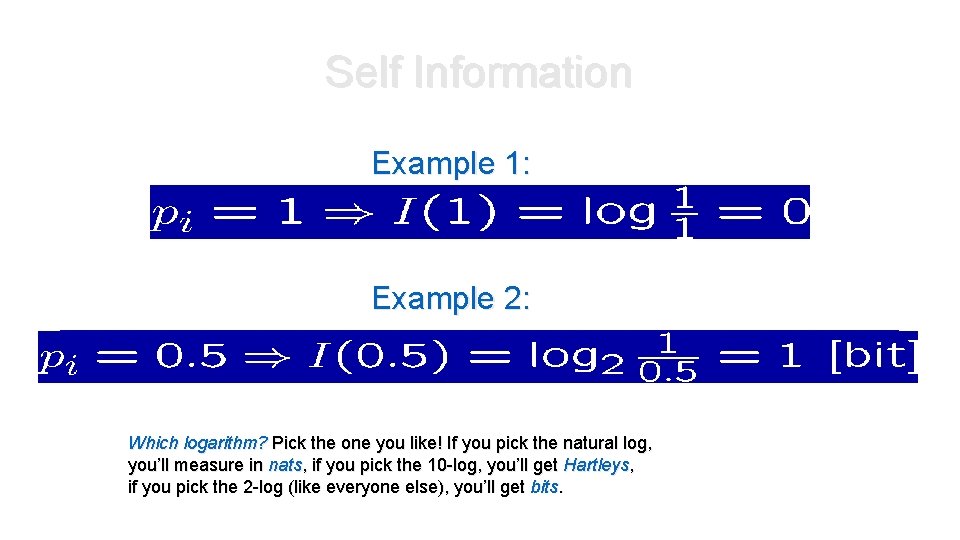
Self Information Example 1: Example 2: Which logarithm? Pick the one you like! If you pick the natural log, you’ll measure in nats, if you pick the 10 -log, you’ll get Hartleys, if you pick the 2 -log (like everyone else), you’ll get bits.

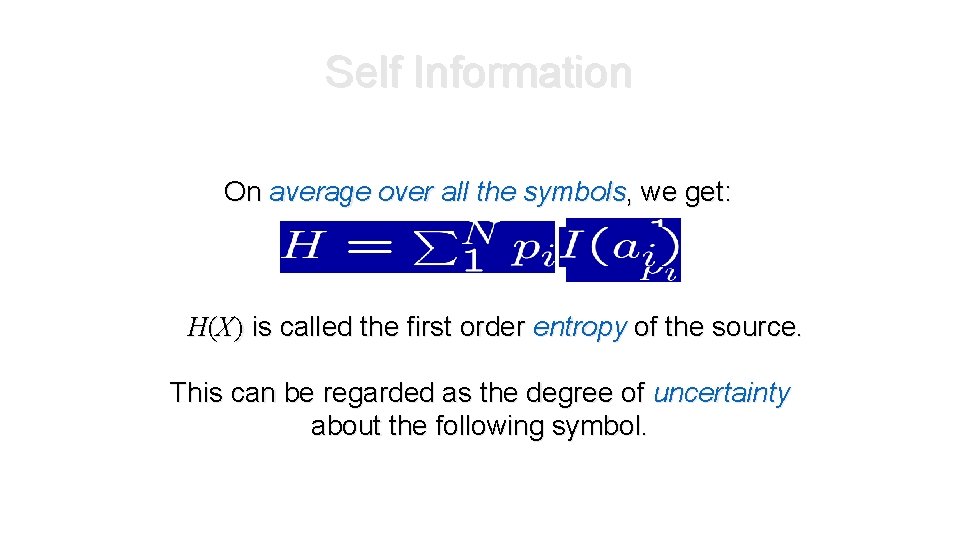
Self Information On average over all the symbols, we get: H(X) is called the first order entropy of the source. This can be regarded as the degree of uncertainty about the following symbol.

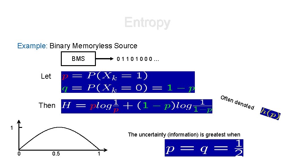
Entropy Example: Binary Memoryless Source BMS 01101000… Let Ofte n de Then note 1 The uncertainty (information) is greatest when 0 0. 5 1 d

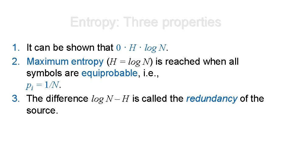
Entropy: Three properties 1. It can be shown that 0 · H · log N. 2. Maximum entropy (H = log N) is reached when all symbols are equiprobable, i. e. , pi = 1/N. 3. The difference log N – H is called the redundancy of the source.

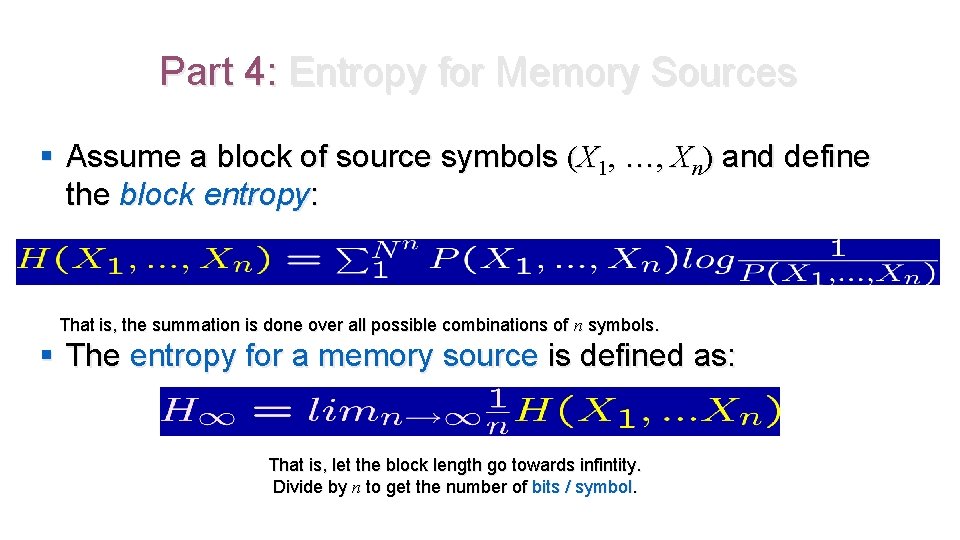
Part 4: Entropy for Memory Sources § Assume a block of source symbols (X 1, …, Xn) and define the block entropy: That is, the summation is done over all possible combinations of n symbols. § The entropy for a memory source is defined as: That is, let the block length go towards infintity. Divide by n to get the number of bits / symbol.

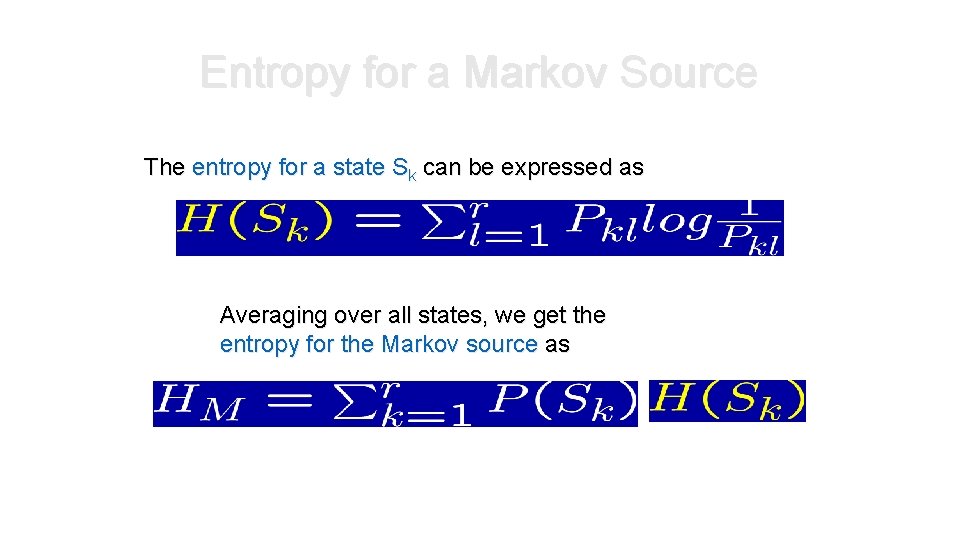
Entropy for a Markov Source The entropy for a state Sk can be expressed as Averaging over all states, we get the entropy for the Markov source as

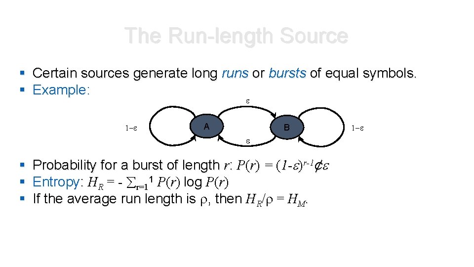
The Run-length Source § Certain sources generate long runs or bursts of equal symbols. § Example: 1 - A B § § § Probability for a burst of length r: P(r) = (1 - )r-1¢ Entropy: HR = - r=11 P(r) log P(r) If the average run length is , then HR/ = HM. 1 -

Part 5: The Source Coding Theorem The entropy is the smallest number of bits allowing error-free representation of the source. Why is this? Let’s take a look on typical sequences!

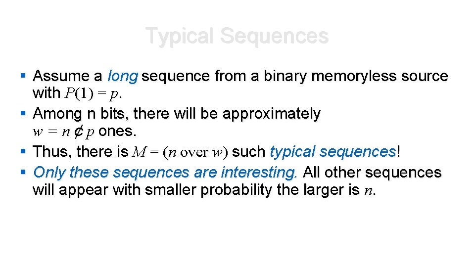
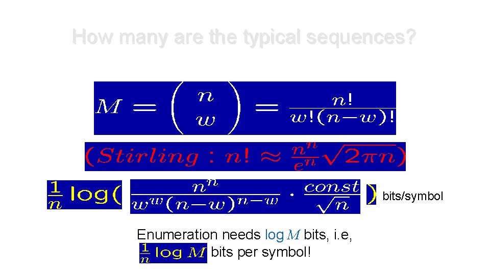
Typical Sequences § Assume a long sequence from a binary memoryless source with P(1) = p. § Among n bits, there will be approximately w = n ¢ p ones. § Thus, there is M = (n over w) such typical sequences! § Only these sequences are interesting. All other sequences will appear with smaller probability the larger is n.

How many are the typical sequences? bits/symbol Enumeration needs log M bits, i. e, bits per symbol!

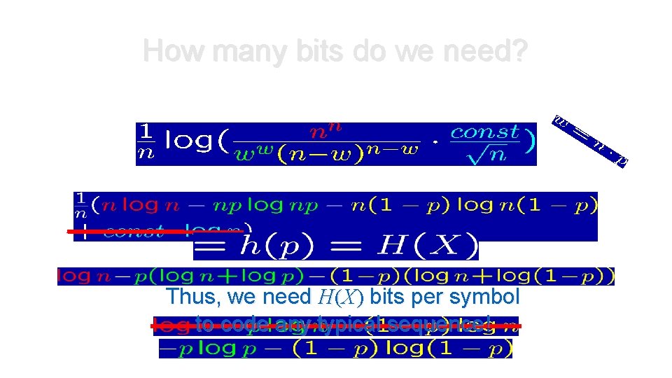
How many bits do we need? Thus, we need H(X) bits per symbol to code any typical sequence!

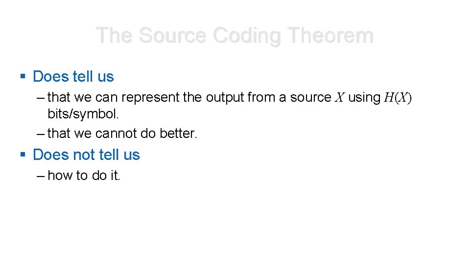
The Source Coding Theorem § Does tell us – that we can represent the output from a source X using H(X) bits/symbol. – that we cannot do better. § Does not tell us – how to do it.

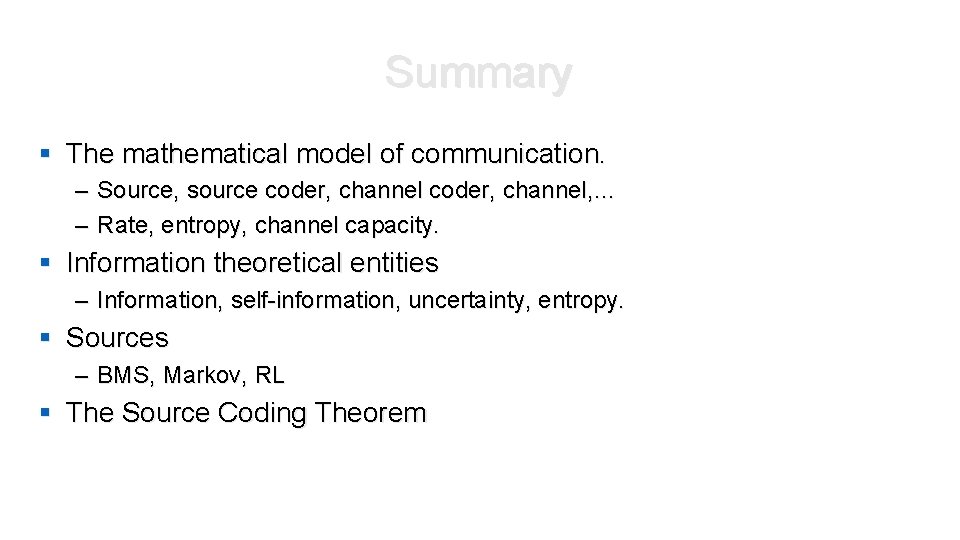
Summary § The mathematical model of communication. – Source, source coder, channel, … – Rate, entropy, channel capacity. § Information theoretical entities – Information, self-information, uncertainty, entropy. § Sources – BMS, Markov, RL § The Source Coding Theorem

UNIT III Baseband Transmission

Sources of Error in received Signal • Major sources of errors: • Thermal noise (AWGN) • disturbs the signal in an additive fashion (Additive) • has flat spectral density for all frequencies of interest (White) • is modeled by Gaussian random process (Gaussian Noise) • Inter-Symbol Interference (ISI) • Due to the filtering effect of transmitter, channel and receiver, symbols are “smeared”.

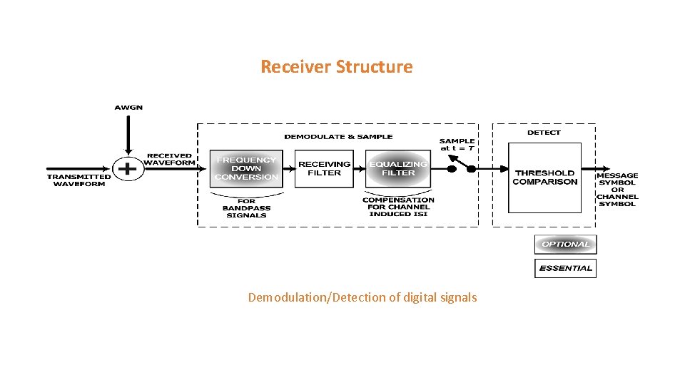
Receiver Structure Demodulation/Detection of digital signals

Receiver Structure contd • The digital receiver performs two basic functions: • Demodulation • Detection • Why demodulate a baseband signal? ? ? • Channel and the transmitter’s filter causes ISI which “smears” the transmitted pulses • Required to recover a waveform to be sampled at t = n. T. • Detection • decision-making process of selecting possible digital symbol

Important Observation • Detection process for bandpass signals is similar to that of baseband signals. WHY? ? ? • Received signal for bandpass signals is converted to baseband before detecting • Bandpass signals are heterodyned to baseband signals • Heterodyning refers to the process of frequency conversion or mixing that yields a spectral shift in frequency. • For linear system mathematics for detection remains same even with the shift in frequency

Steps in designing the receiver • Find optimum solution for receiver design with the following goals: 1. 2. • Maximize SNR Minimize ISI Steps in design: • • Model the received signal Find separate solutions for each of the goals.

Detection of Binary Signal in Gaussian Noise • The recovery of signal at the receiver consist of two parts • Filter • Reduces the received signal to a single variable z(T) • z(T) is called the test statistics • Detector (or decision circuit) • Compares the z(T) to some threshold level 0 , i. e. , possible binary hypothesis where H 1 and H 0 are the two

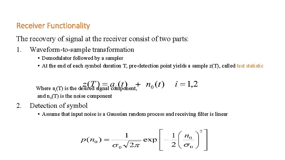
Receiver Functionality The recovery of signal at the receiver consist of two parts: 1. Waveform-to-sample transformation • Demodulator followed by a sampler • At the end of each symbol duration T, pre-detection point yields a sample z(T), called test statistic Where ai(T) is the desired signal component, and no(T) is the noise component 2. Detection of symbol • Assume that input noise is a Gaussian random process and receiving filter is linear

Finding optimized filter for AWGN channel Assuming Channel with response equal to impulse function

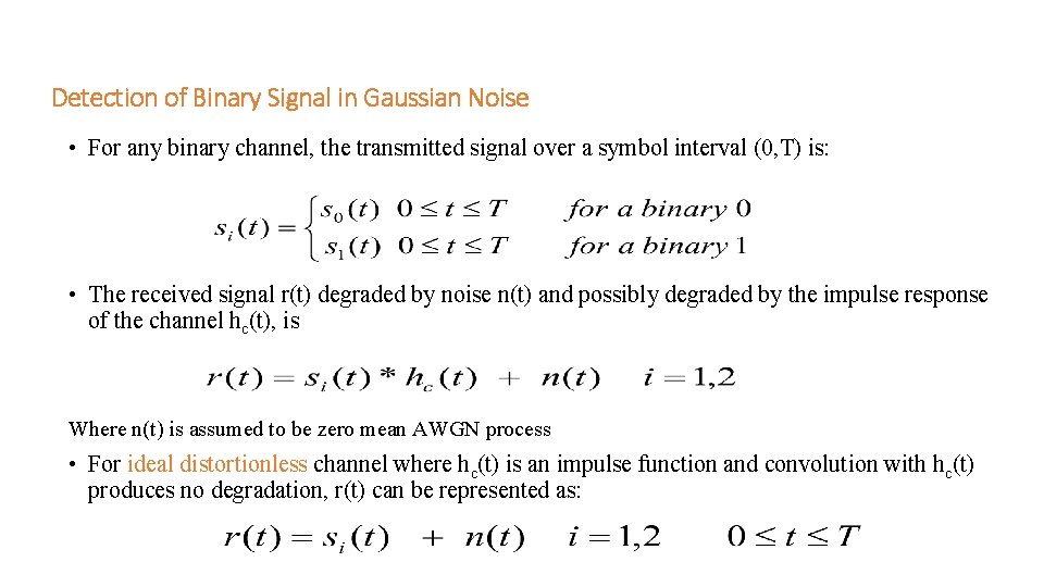
Detection of Binary Signal in Gaussian Noise • For any binary channel, the transmitted signal over a symbol interval (0, T) is: • The received signal r(t) degraded by noise n(t) and possibly degraded by the impulse response of the channel hc(t), is Where n(t) is assumed to be zero mean AWGN process • For ideal distortionless channel where hc(t) is an impulse function and convolution with hc(t) produces no degradation, r(t) can be represented as:

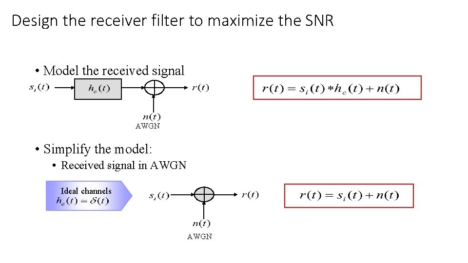
Design the receiver filter to maximize the SNR • Model the received signal AWGN • Simplify the model: • Received signal in AWGN Ideal channels AWGN

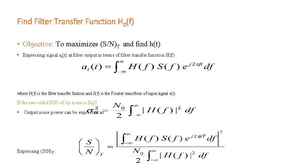
Find Filter Transfer Function H 0(f) • Objective: To maximizes (S/N)T and find h(t) • Expressing signal ai(t) at filter output in terms of filter transfer function H(f) where H(f) is the filter transfer funtion and S(f) is the Fourier transform of input signal s(t) If the two sided PSD of i/p noise is N 0/2 • Output noise power can be expressed as: Expressing (S/N)T :

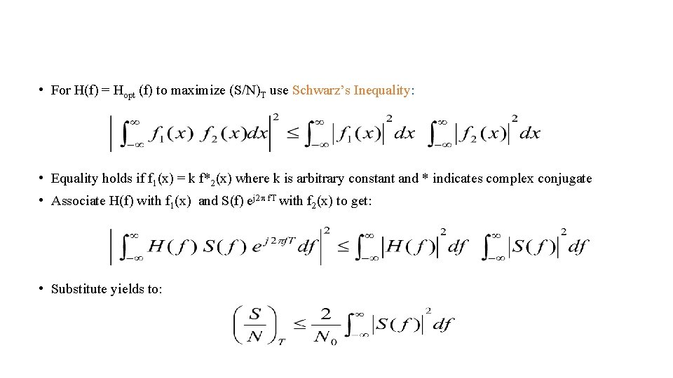
• For H(f) = Hopt (f) to maximize (S/N)T use Schwarz’s Inequality: • Equality holds if f 1(x) = k f*2(x) where k is arbitrary constant and * indicates complex conjugate • Associate H(f) with f 1(x) and S(f) ej 2 f. T with f 2(x) to get: • Substitute yields to:

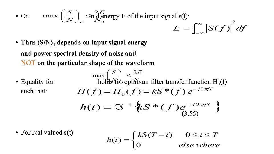
• Or and energy E of the input signal s(t): • Thus (S/N)T depends on input signal energy and power spectral density of noise and NOT on the particular shape of the waveform • Equality for such that: holds for optimum filter transfer function H 0(f) (3. 55) • For real valued s(t):

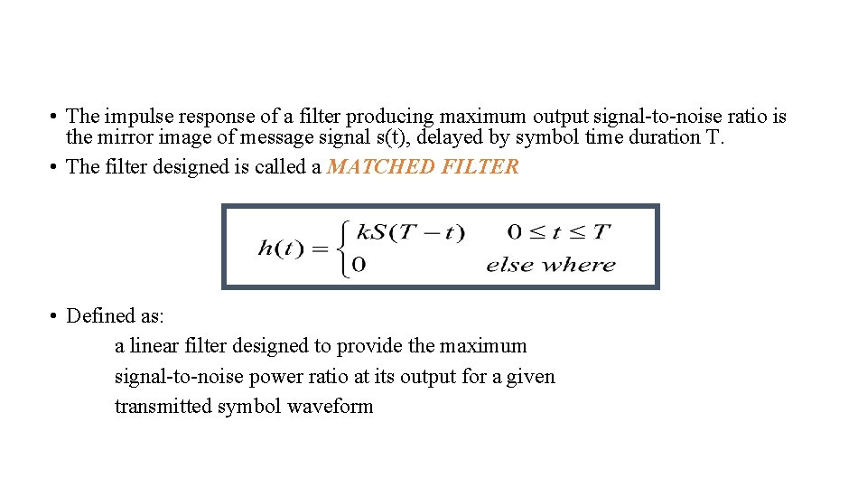
• The impulse response of a filter producing maximum output signal-to-noise ratio is the mirror image of message signal s(t), delayed by symbol time duration T. • The filter designed is called a MATCHED FILTER • Defined as: a linear filter designed to provide the maximum signal-to-noise power ratio at its output for a given transmitted symbol waveform

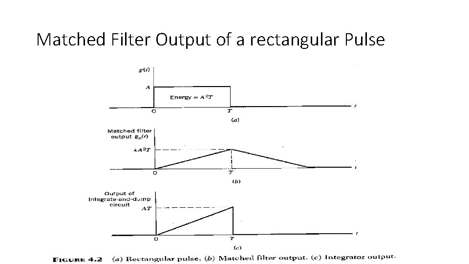
Matched Filter Output of a rectangular Pulse

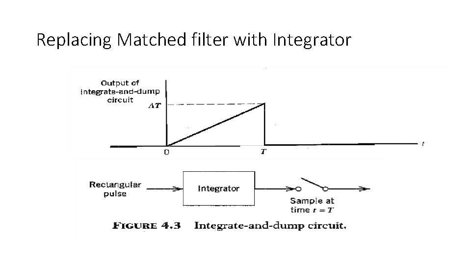
Replacing Matched filter with Integrator

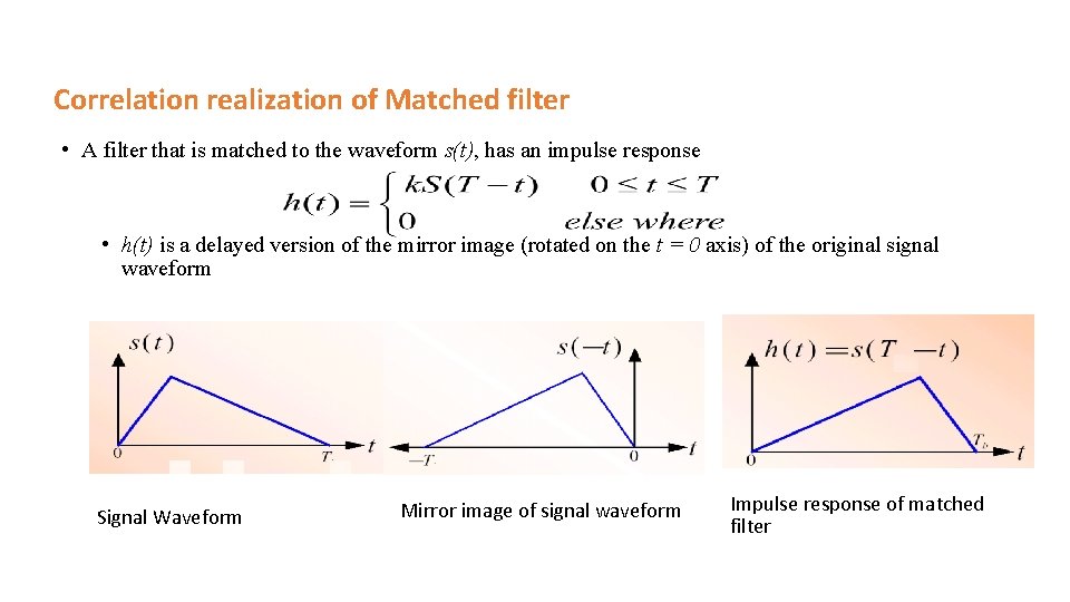
Correlation realization of Matched filter • A filter that is matched to the waveform s(t), has an impulse response • h(t) is a delayed version of the mirror image (rotated on the t = 0 axis) of the original signal waveform Signal Waveform Mirror image of signal waveform Impulse response of matched filter

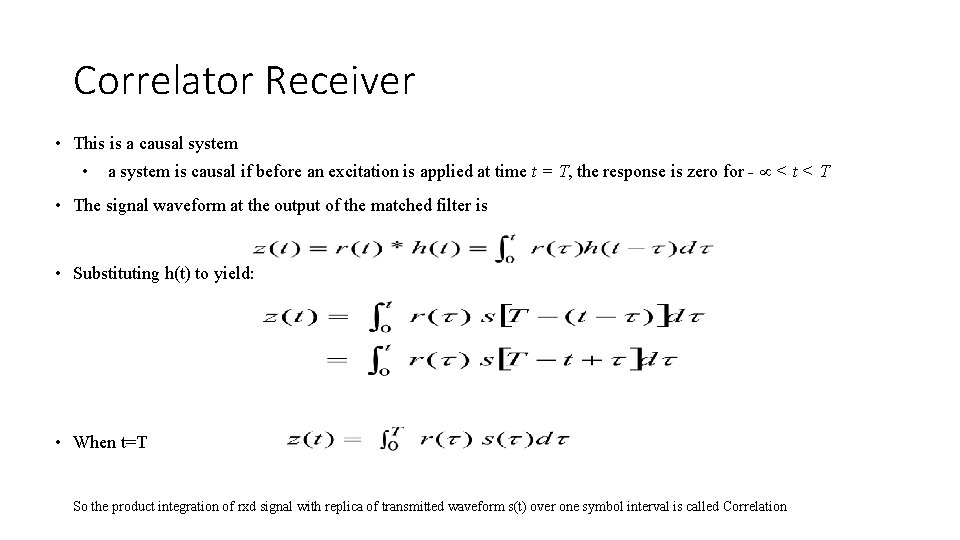
Correlator Receiver • This is a causal system • a system is causal if before an excitation is applied at time t = T, the response is zero for - < t < T • The signal waveform at the output of the matched filter is • Substituting h(t) to yield: • When t=T So the product integration of rxd signal with replica of transmitted waveform s(t) over one symbol interval is called Correlation

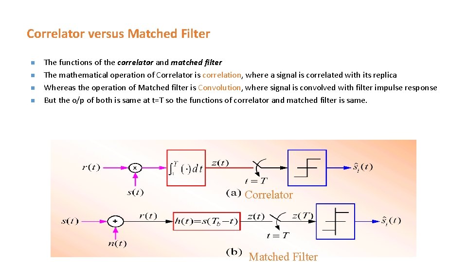
Correlator versus Matched Filter n n The functions of the correlator and matched filter The mathematical operation of Correlator is correlation, where a signal is correlated with its replica Whereas the operation of Matched filter is Convolution, where signal is convolved with filter impulse response But the o/p of both is same at t=T so the functions of correlator and matched filter is same. Correlator Matched Filter

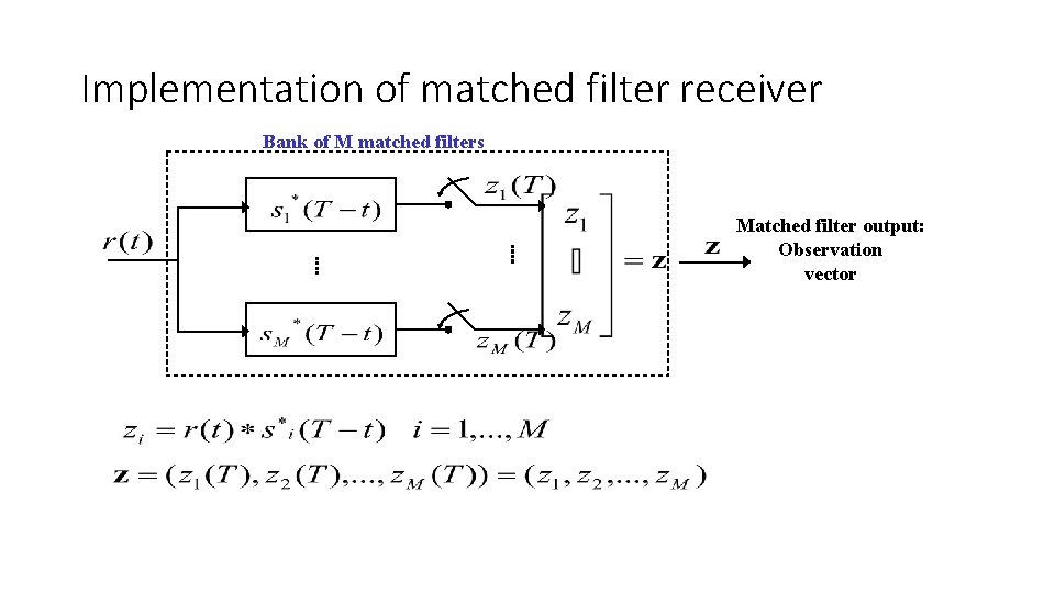
Implementation of matched filter receiver Bank of M matched filters Matched filter output: Observation vector

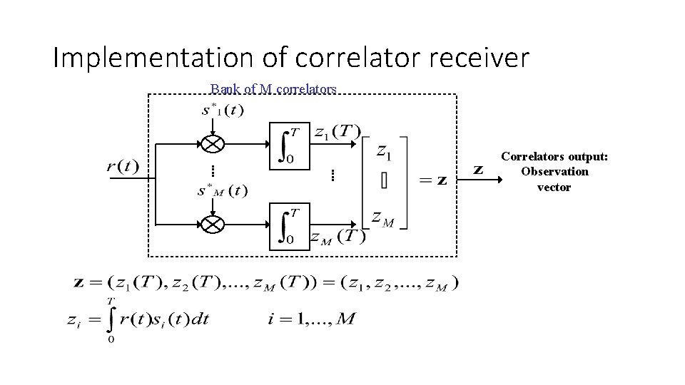
Implementation of correlator receiver Bank of M correlators Correlators output: Observation vector

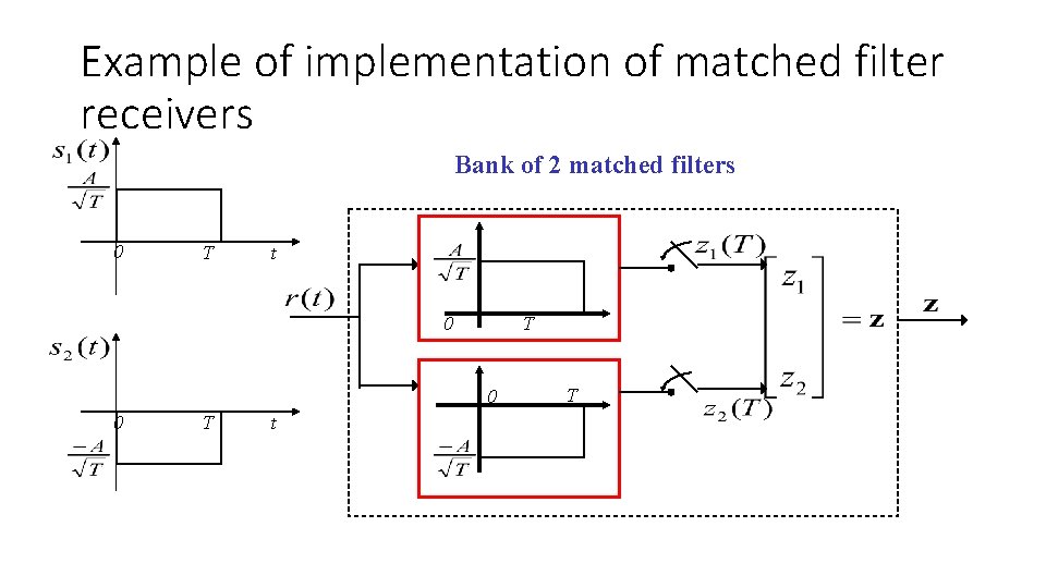
Example of implementation of matched filter receivers Bank of 2 matched filters 0 T t 0 T 0 0 T t T

Detection Max. Likelihood Detector Probability of Error

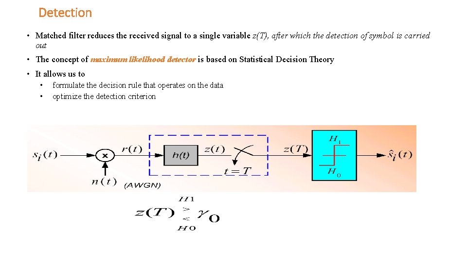
Detection • Matched filter reduces the received signal to a single variable z(T), after which the detection of symbol is carried out • The concept of maximum likelihood detector is based on Statistical Decision Theory • It allows us to • • formulate the decision rule that operates on the data optimize the detection criterion

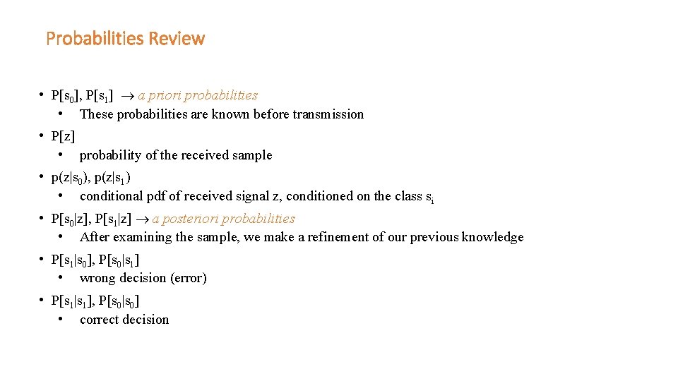
Probabilities Review • P[s 0], P[s 1] a priori probabilities • These probabilities are known before transmission • P[z] • probability of the received sample • p(z|s 0), p(z|s 1) • conditional pdf of received signal z, conditioned on the class si • P[s 0|z], P[s 1|z] a posteriori probabilities • After examining the sample, we make a refinement of our previous knowledge • P[s 1|s 0], P[s 0|s 1] • wrong decision (error) • P[s 1|s 1], P[s 0|s 0] • correct decision

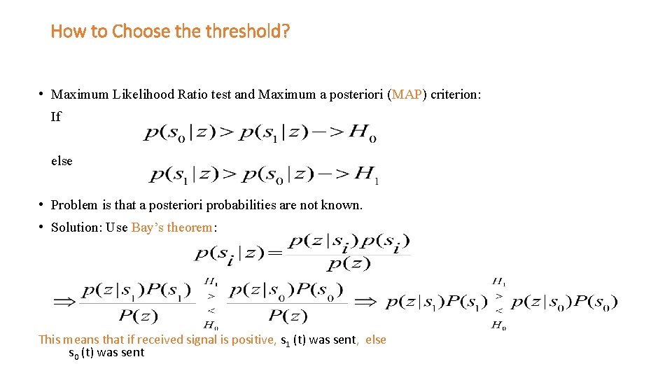
How to Choose threshold? • Maximum Likelihood Ratio test and Maximum a posteriori (MAP) criterion: If else • Problem is that a posteriori probabilities are not known. • Solution: Use Bay’s theorem: This means that if received signal is positive, s 1 (t) was sent, else s 0 (t) was sent

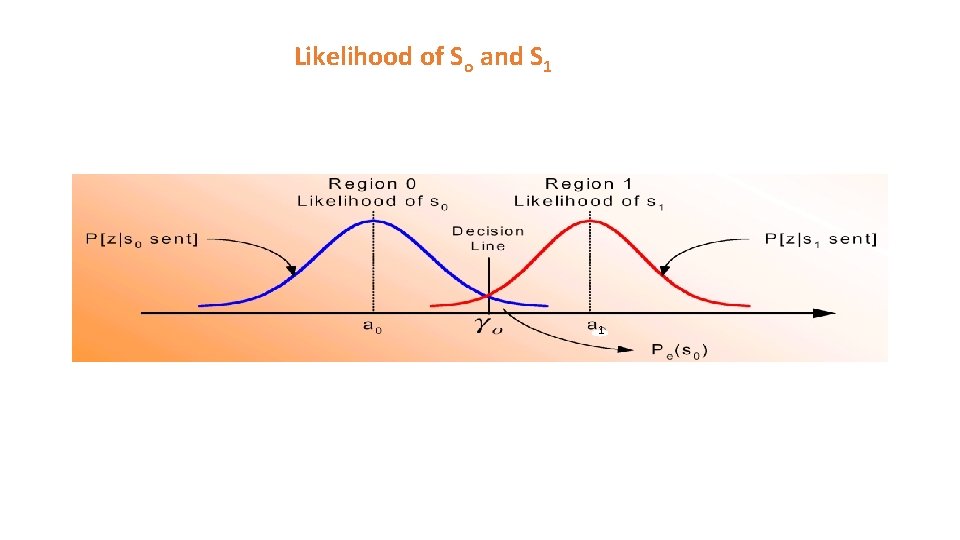
Likelihood of So and S 1 1

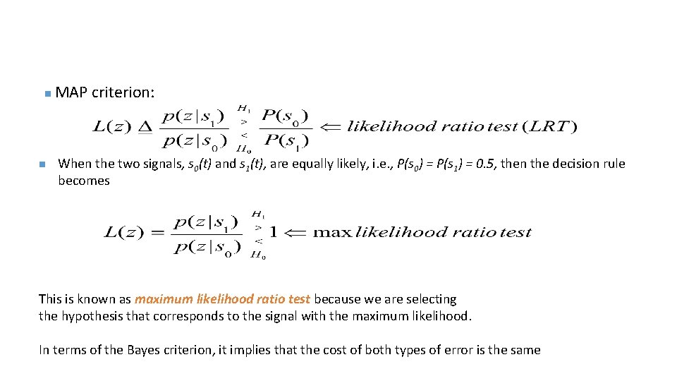
n n MAP criterion: When the two signals, s 0(t) and s 1(t), are equally likely, i. e. , P(s 0) = P(s 1) = 0. 5, then the decision rule becomes This is known as maximum likelihood ratio test because we are selecting the hypothesis that corresponds to the signal with the maximum likelihood. In terms of the Bayes criterion, it implies that the cost of both types of error is the same

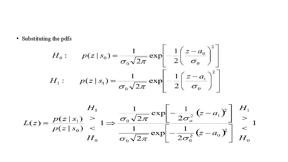
• Substituting the pdfs

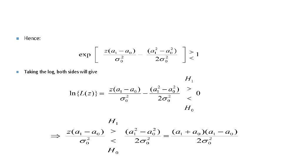
n Hence: n Taking the log, both sides will give

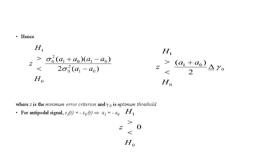
• Hence where z is the minimum error criterion and 0 is optimum threshold • For antipodal signal, s 1(t) = - s 0 (t) a 1 = - a 0

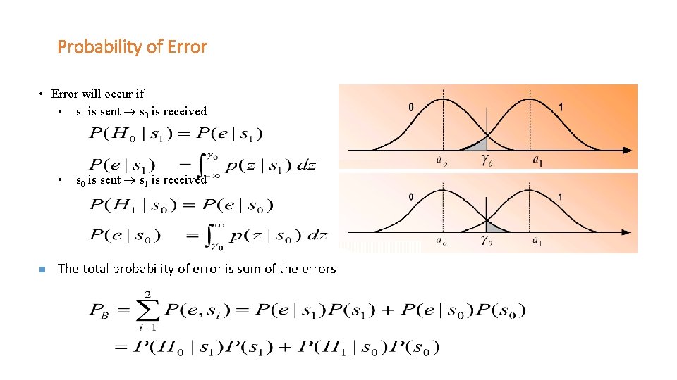
Probability of Error • Error will occur if • s 1 is sent s 0 is received • n s 0 is sent s 1 is received The total probability of error is sum of the errors

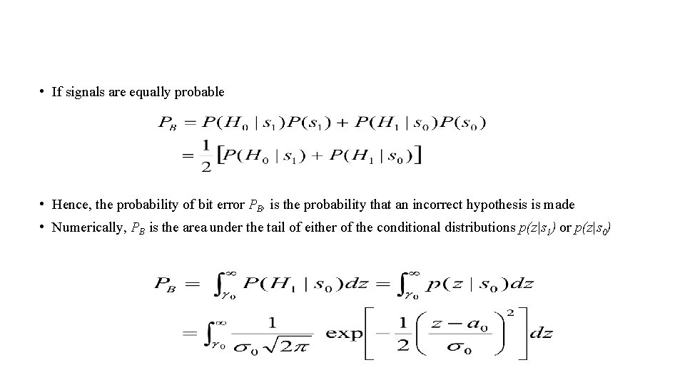
• If signals are equally probable • Hence, the probability of bit error PB, is the probability that an incorrect hypothesis is made • Numerically, PB is the area under the tail of either of the conditional distributions p(z|s 1) or p(z|s 0)

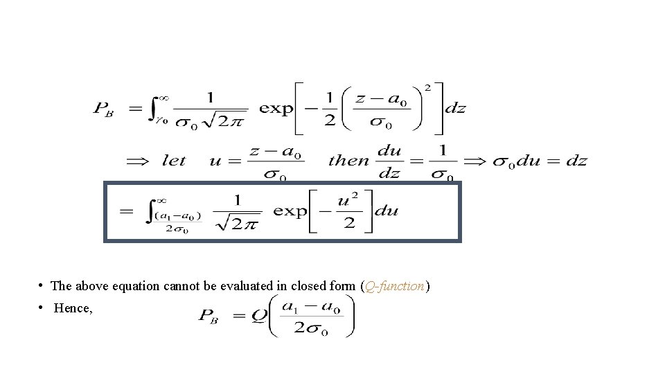
• The above equation cannot be evaluated in closed form (Q-function) • Hence,

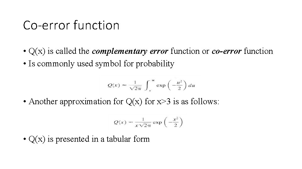
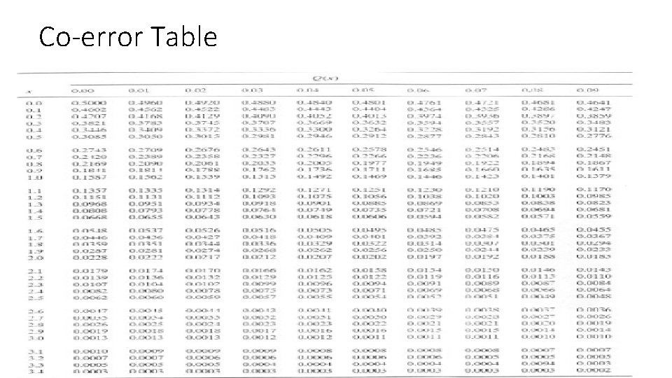
Co-error function • Q(x) is called the complementary error function or co-error function • Is commonly used symbol for probability • Another approximation for Q(x) for x>3 is as follows: • Q(x) is presented in a tabular form

Co-error Table

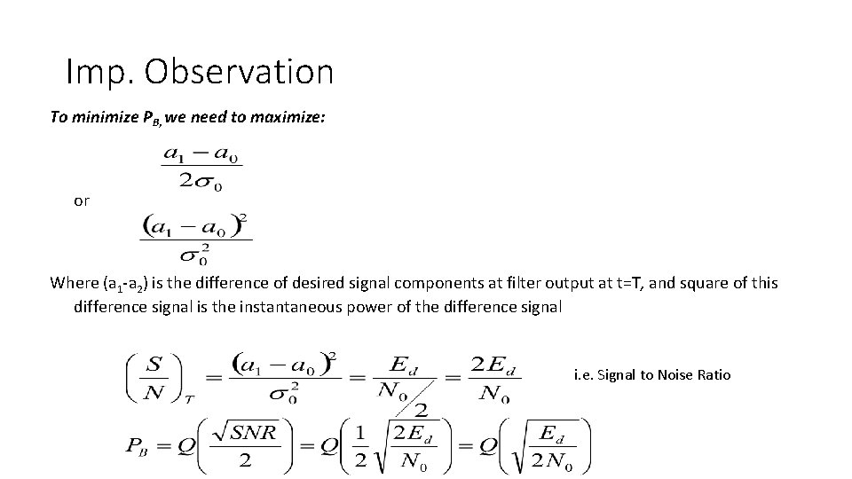
Imp. Observation To minimize PB, we need to maximize: or Where (a 1 -a 2) is the difference of desired signal components at filter output at t=T, and square of this difference signal is the instantaneous power of the difference signal i. e. Signal to Noise Ratio

Unit IV Digital modulation techniques

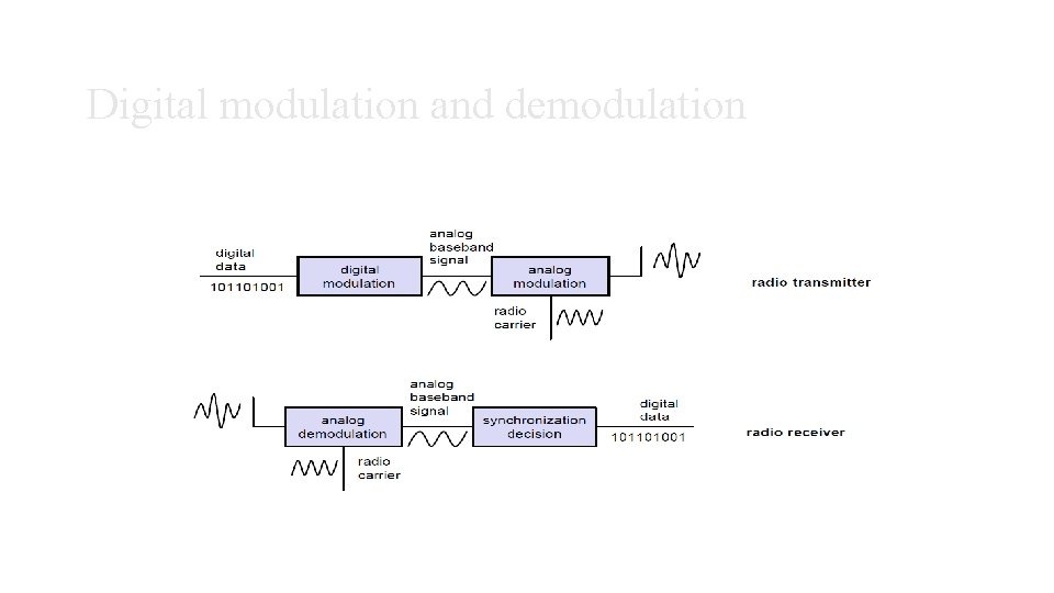
Digital modulation and demodulation

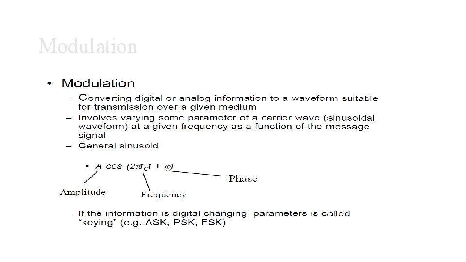
Modulation

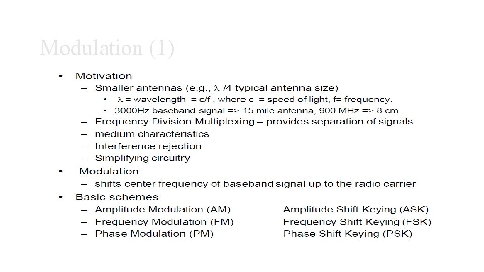
Modulation (1)

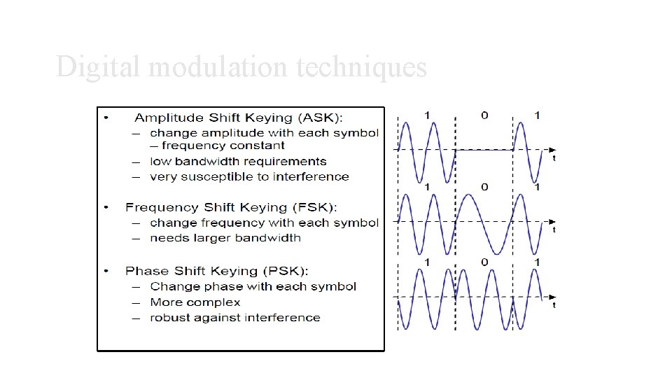
Digital modulation techniques

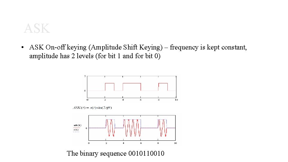
ASK • ASK On-off keying (Amplitude Shift Keying) – frequency is kept constant, amplitude has 2 levels (for bit 1 and for bit 0) The binary sequence 0010110010

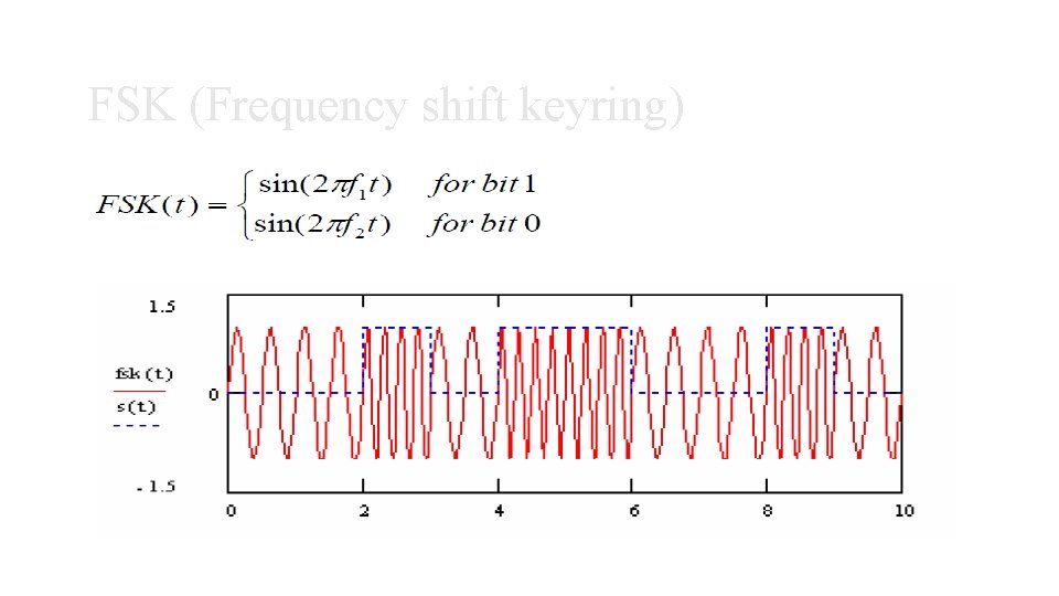
FSK (Frequency shift keyring)

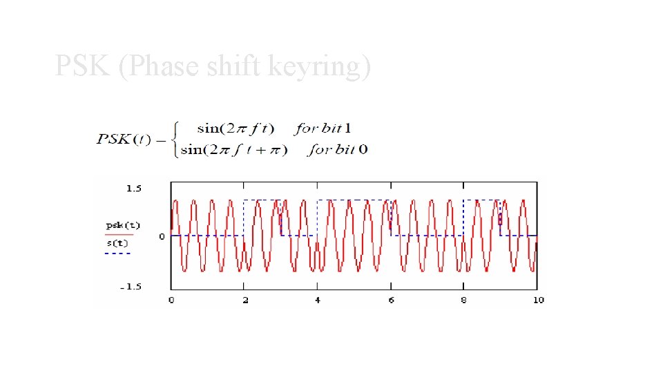
PSK (Phase shift keyring)

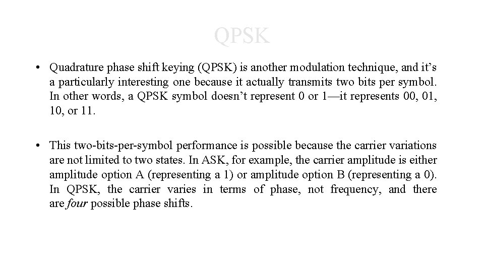
QPSK • Quadrature phase shift keying (QPSK) is another modulation technique, and it’s a particularly interesting one because it actually transmits two bits per symbol. In other words, a QPSK symbol doesn’t represent 0 or 1—it represents 00, 01, 10, or 11. • This two-bits-per-symbol performance is possible because the carrier variations are not limited to two states. In ASK, for example, the carrier amplitude is either amplitude option A (representing a 1) or amplitude option B (representing a 0). In QPSK, the carrier varies in terms of phase, not frequency, and there are four possible phase shifts.

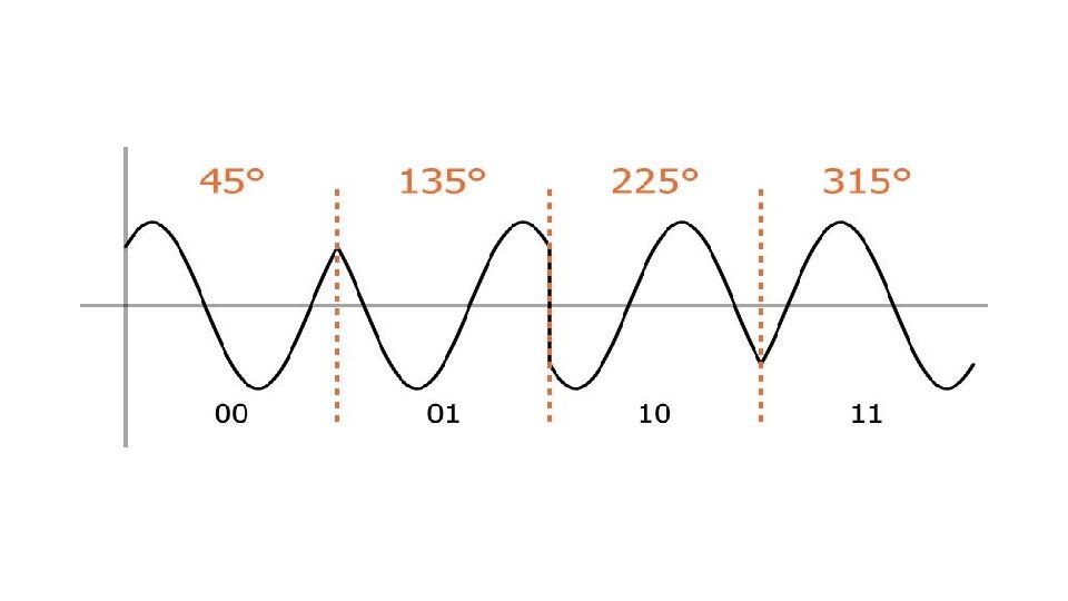
• We can intuitively determine what these four possible phase shifts should be: First we recall that modulation is only the beginning of the communication process; the receiver needs to be able to extract the original information from the modulated signal. Next, it makes sense to seek maximum separation between the four phase options, so that the receiver has less difficulty distinguishing one state from another. We have 360° of phase to work with and four phase states, and thus the separation should be 360°/4 = 90°. So our four QPSK phase shifts are 45°, 135°, 225°, and 315°.

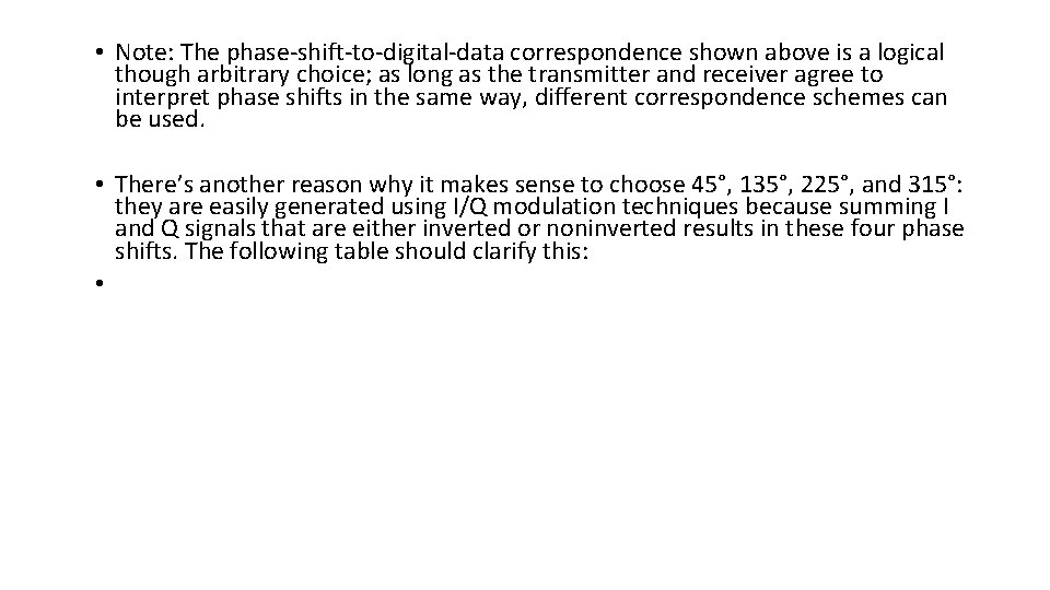
• Note: The phase-shift-to-digital-data correspondence shown above is a logical though arbitrary choice; as long as the transmitter and receiver agree to interpret phase shifts in the same way, different correspondence schemes can be used. • There’s another reason why it makes sense to choose 45°, 135°, 225°, and 315°: they are easily generated using I/Q modulation techniques because summing I and Q signals that are either inverted or noninverted results in these four phase shifts. The following table should clarify this: •

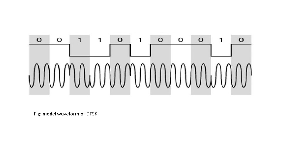
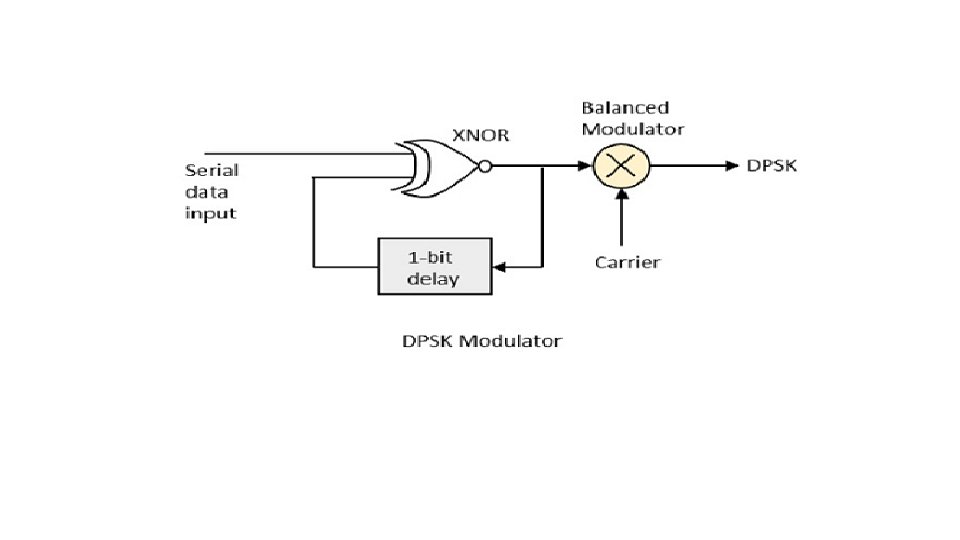
DPSK • In Differential Phase Shift Keying (DPSK) the phase of the modulated signal is shifted relative to the previous signal element. No reference signal is considered here. The signal phase follows the high or low state of the previous element. This DPSK technique doesn’t need a reference oscillator.

Fig: model waveform of DPSK

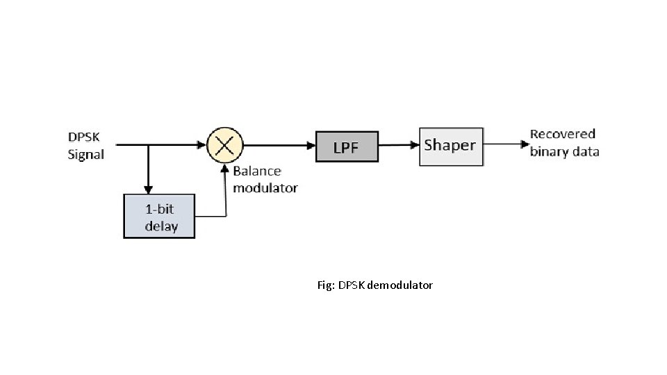
Fig: DPSK demodulator

Spread spectrum modulation. Unit 5

Outlines • • Model of Spread spectrum PN sequence generation DSSS Performance parameter of DSSS FHSS Ranging using DSSS Comparison of slow and fast frequency hopping. Synchronization in spread spectrum system.

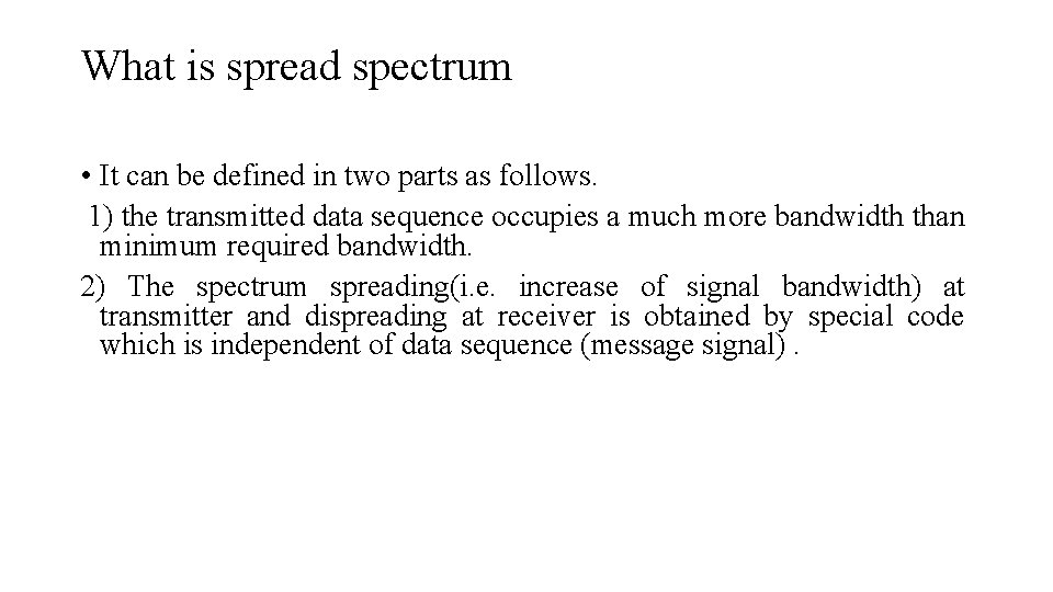
What is spread spectrum • It can be defined in two parts as follows. 1) the transmitted data sequence occupies a much more bandwidth than minimum required bandwidth. 2) The spectrum spreading(i. e. increase of signal bandwidth) at transmitter and dispreading at receiver is obtained by special code which is independent of data sequence (message signal).

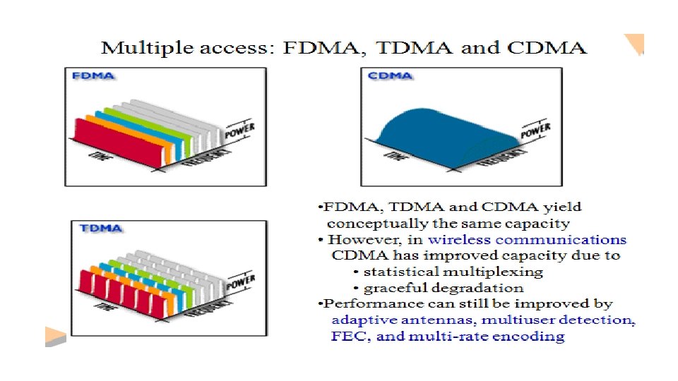
Applications • Antijamming applications for military applications • Low probability of intercept • Mobile communications • Secured communications • Distance measurements • Selective calling • CDMA communication

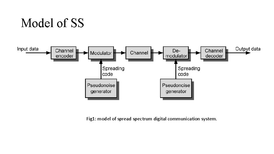
Model of SS Fig 1: model of spread spectrum digital communication system.

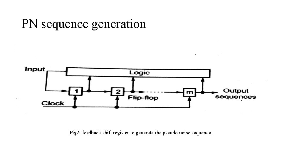
PN sequence generation Fig 2: feedback shift register to generate the pseudo noise sequence.

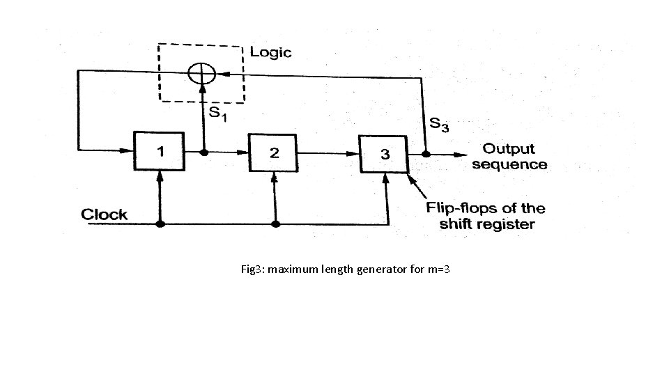
• Maximum length sequence: when PN sequence generated by linear feedback shift register has the length of 2^m -1, it is called maximum length sequence. • Properties of Maximum length sequence: 1) Balance property 2) Run property 3) Correlation property.

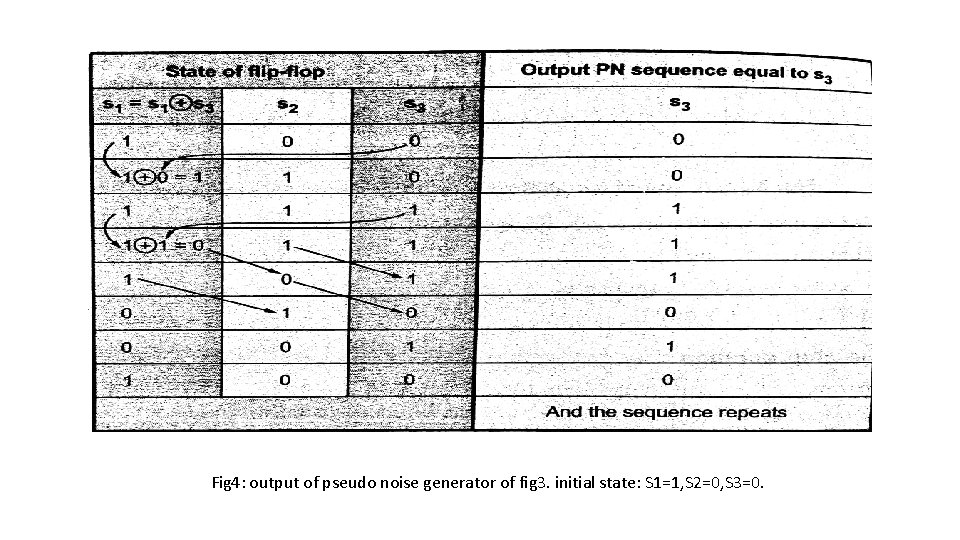
Fig 3: maximum length generator for m=3

Fig 4: output of pseudo noise generator of fig 3. initial state: S 1=1, S 2=0, S 3=0.

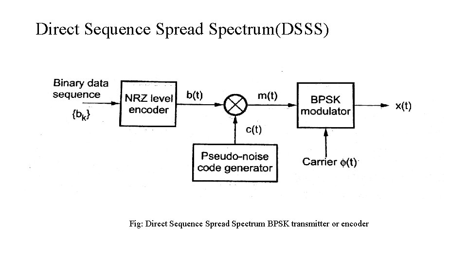
Direct Sequence Spread Spectrum(DSSS) Fig: Direct Sequence Spread Spectrum BPSK transmitter or encoder

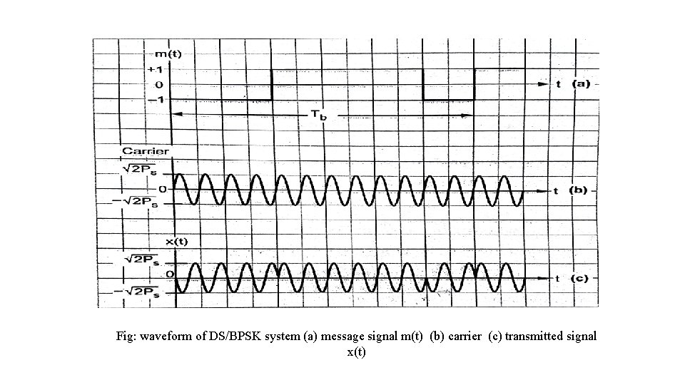
Fig: waveform of DS/BPSK system (a) message signal m(t) (b) carrier (c) transmitted signal x(t)

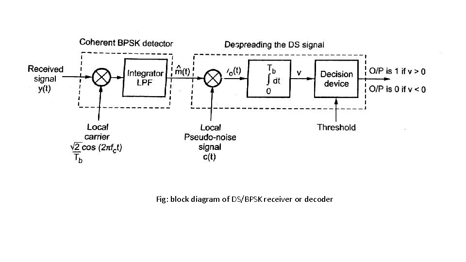
Fig: block diagram of DS/BPSK receiver or decoder

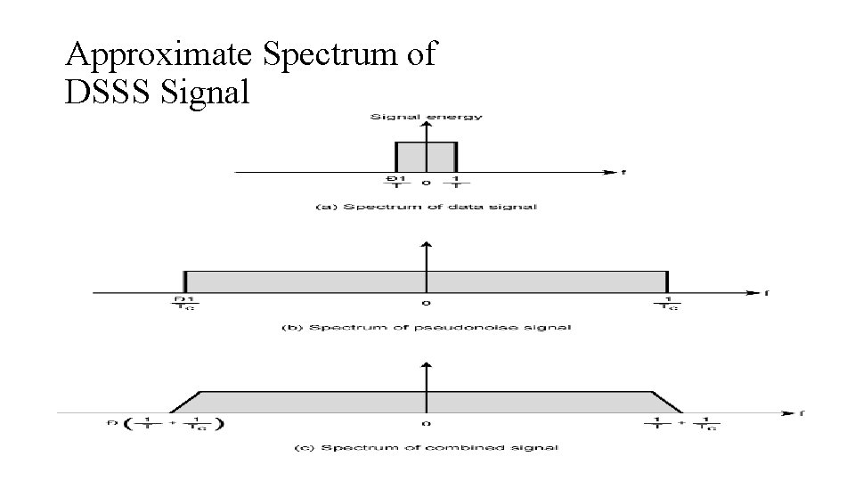
Approximate Spectrum of DSSS Signal

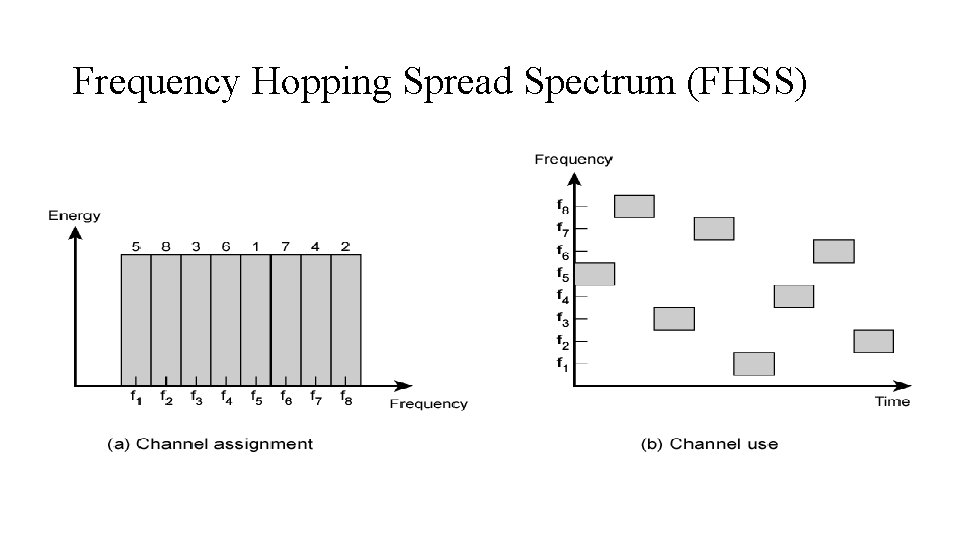
Frequency Hopping Spread Spectrum (FHSS)

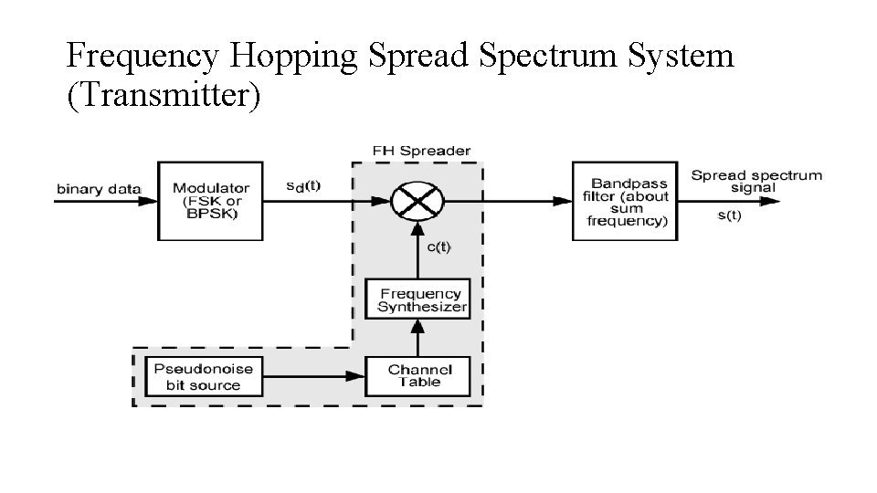
Frequency Hopping Spread Spectrum System (Transmitter)

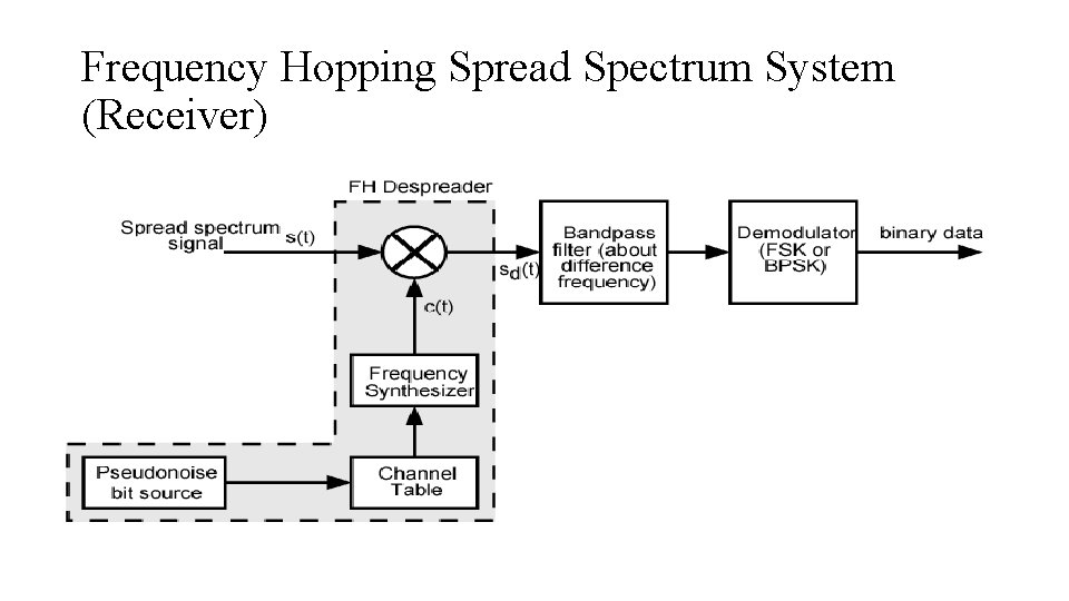
Frequency Hopping Spread Spectrum System (Receiver)

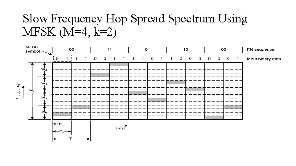
Slow Frequency Hop Spread Spectrum Using MFSK (M=4, k=2)

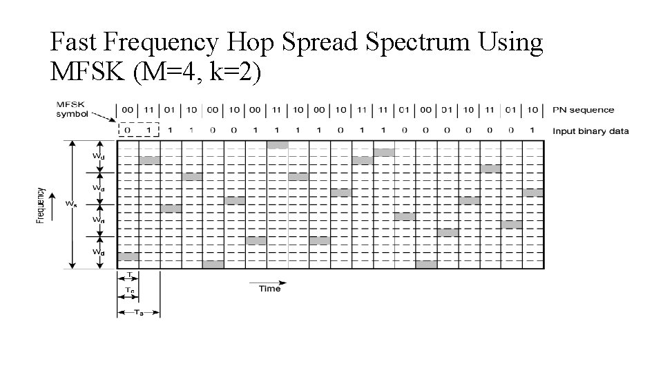
Fast Frequency Hop Spread Spectrum Using MFSK (M=4, k=2)

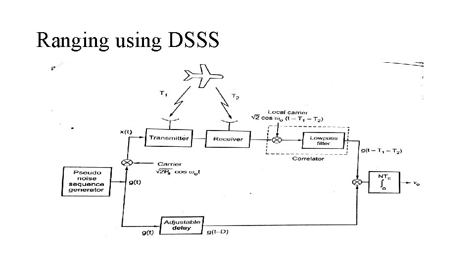
Ranging using DSSS

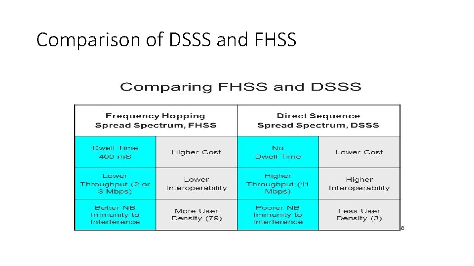
Comparison of DSSS and FHSS

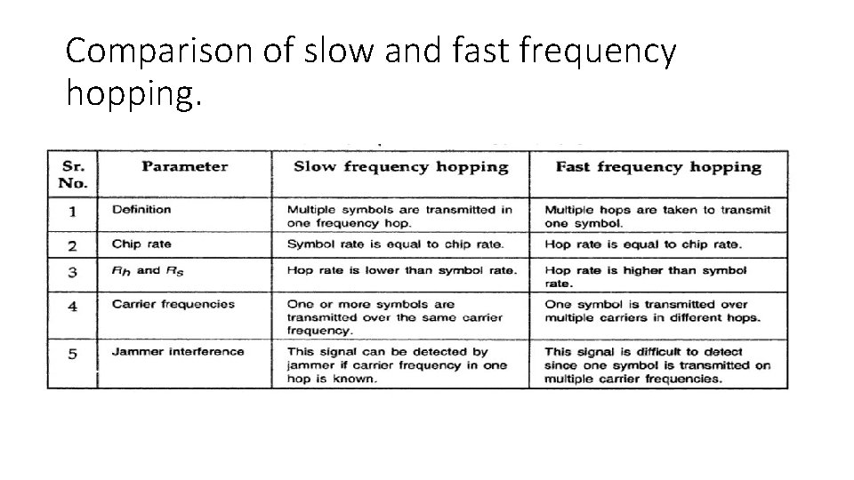
Comparison of slow and fast frequency hopping.

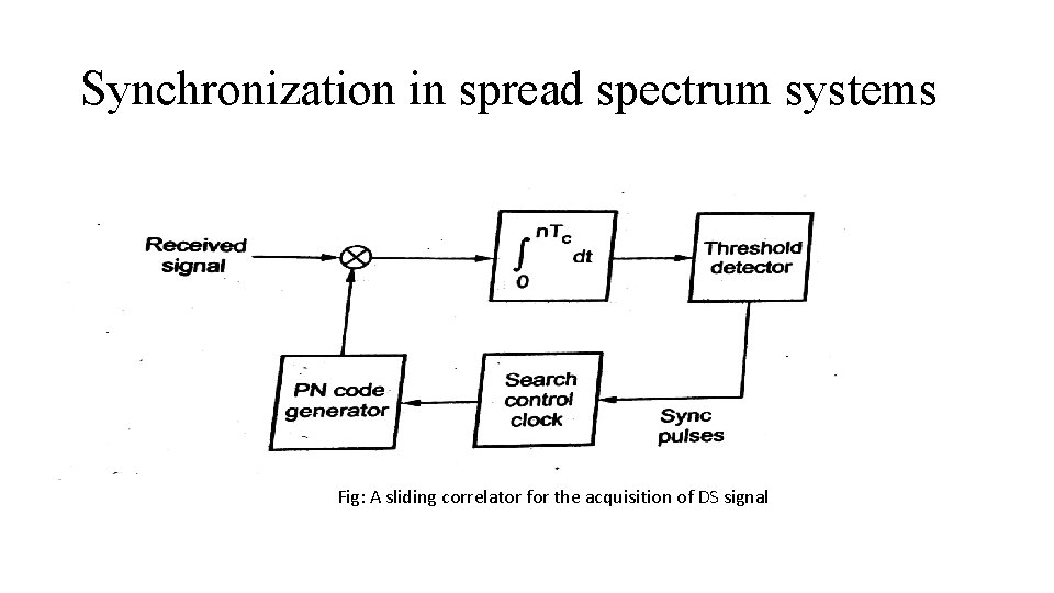
Synchronization in spread spectrum systems Fig: A sliding correlator for the acquisition of DS signal

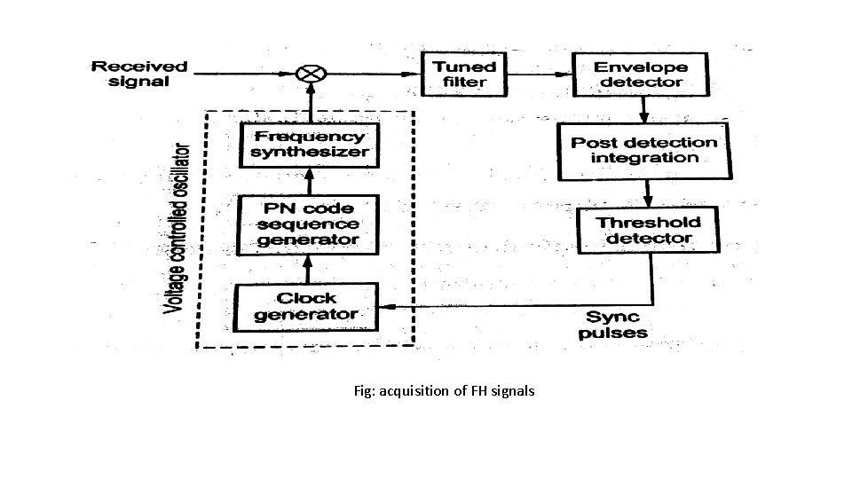
Fig: acquisition of FH signals