UNIT6 Classification and Prediction Lecture Topic Lecture32 What

UNIT-6 Classification and Prediction Lecture Topic *********************** Lecture-32 What is classification? What is prediction? Lecture-33 Issues regarding classification and prediction Lecture-34 Classification by decision tree induction Lecture-35 Bayesian Classification Lecture-36 Classification by backpropagation Lecture-37 Classification based on concepts from association rule mining Lecture-38 Other Classification Methods Lecture-39 Prediction Lecture-40 Classification accuracy

Lecture-32 What is classification? What is prediction?

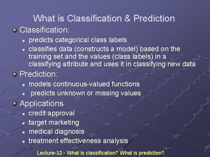
What is Classification & Prediction Classification: n n predicts categorical class labels classifies data (constructs a model) based on the training set and the values (class labels) in a classifying attribute and uses it in classifying new data Prediction: n n models continuous-valued functions predicts unknown or missing values Applications n n credit approval target marketing medical diagnosis treatment effectiveness analysis Lecture-32 - What is classification? What is prediction?

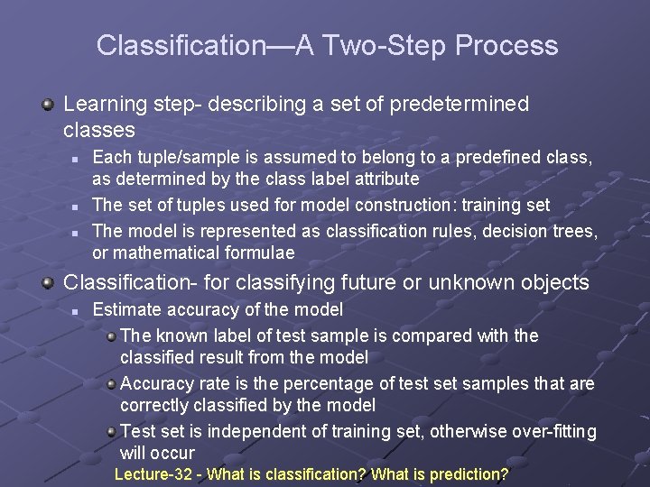
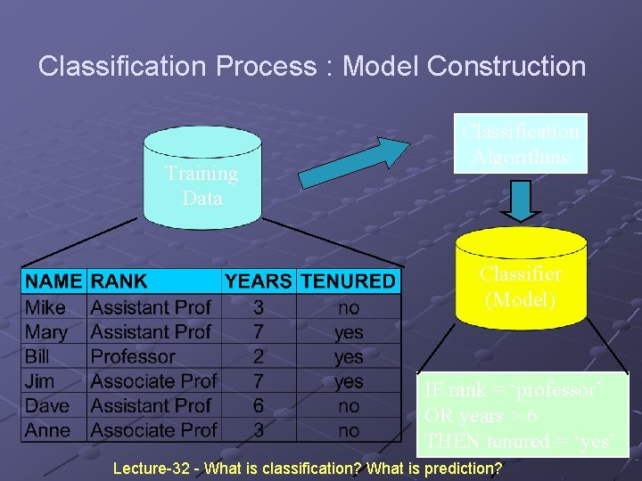
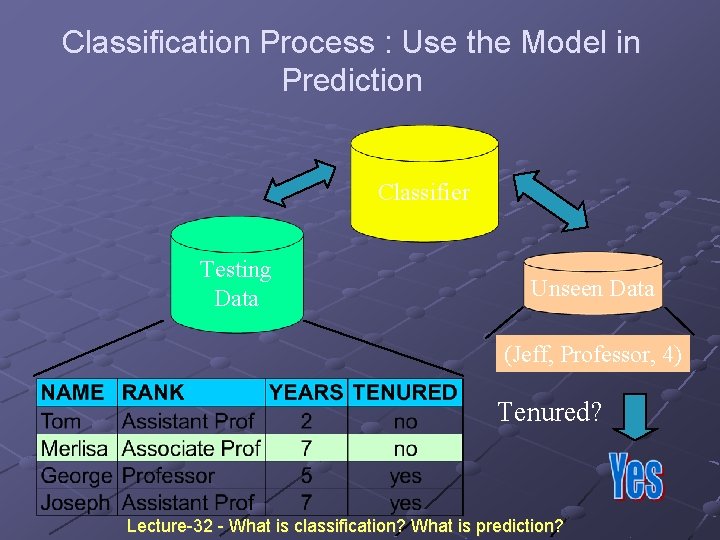
Classification—A Two-Step Process Learning step- describing a set of predetermined classes n n n Each tuple/sample is assumed to belong to a predefined class, as determined by the class label attribute The set of tuples used for model construction: training set The model is represented as classification rules, decision trees, or mathematical formulae Classification- for classifying future or unknown objects n Estimate accuracy of the model The known label of test sample is compared with the classified result from the model Accuracy rate is the percentage of test set samples that are correctly classified by the model Test set is independent of training set, otherwise over-fitting will occur Lecture-32 - What is classification? What is prediction?

Classification Process : Model Construction Training Data Classification Algorithms Classifier (Model) IF rank = ‘professor’ OR years > 6 THEN tenured = ‘yes’ Lecture-32 - What is classification? What is prediction?

Classification Process : Use the Model in Prediction Classifier Testing Data Unseen Data (Jeff, Professor, 4) Tenured? Lecture-32 - What is classification? What is prediction?

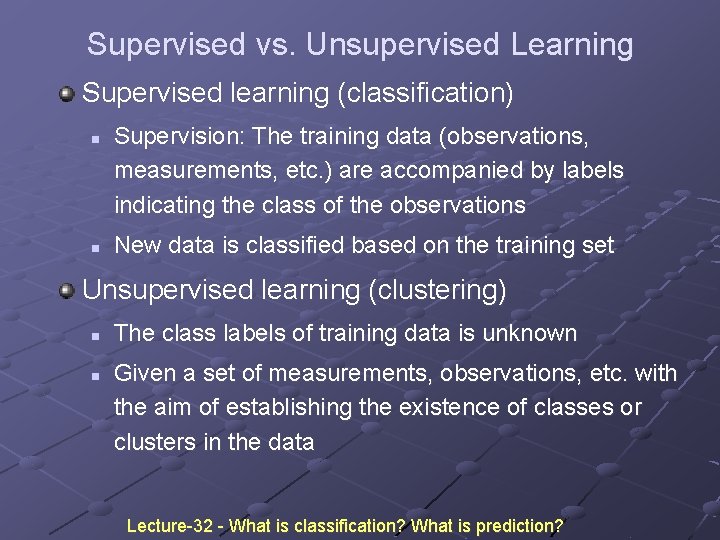
Supervised vs. Unsupervised Learning Supervised learning (classification) n n Supervision: The training data (observations, measurements, etc. ) are accompanied by labels indicating the class of the observations New data is classified based on the training set Unsupervised learning (clustering) n n The class labels of training data is unknown Given a set of measurements, observations, etc. with the aim of establishing the existence of classes or clusters in the data Lecture-32 - What is classification? What is prediction?

Lecture-33 Issues regarding classification and prediction

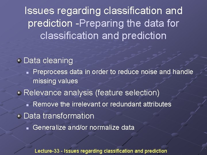
Issues regarding classification and prediction -Preparing the data for classification and prediction Data cleaning n Preprocess data in order to reduce noise and handle missing values Relevance analysis (feature selection) n Remove the irrelevant or redundant attributes Data transformation n Generalize and/or normalize data Lecture-33 - Issues regarding classification and prediction

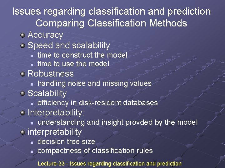
Issues regarding classification and prediction Comparing Classification Methods Accuracy Speed and scalability n n time to construct the model time to use the model Robustness n handling noise and missing values Scalability n efficiency in disk-resident databases Interpretability: n understanding and insight provded by the model interpretability n n decision tree size compactness of classification rules Lecture-33 - Issues regarding classification and prediction

Lecture-34 Classification by decision tree induction Lecture-34 - Classification by decision tree induction

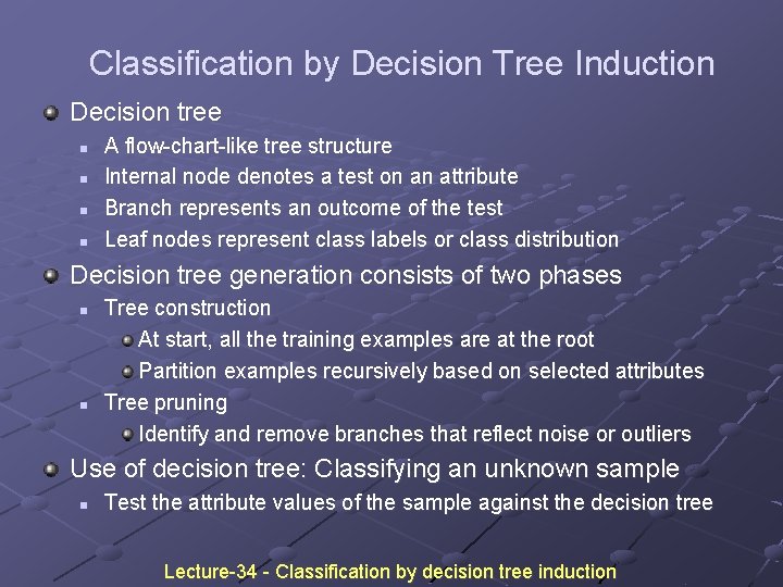
Classification by Decision Tree Induction Decision tree n n A flow-chart-like tree structure Internal node denotes a test on an attribute Branch represents an outcome of the test Leaf nodes represent class labels or class distribution Decision tree generation consists of two phases n n Tree construction At start, all the training examples are at the root Partition examples recursively based on selected attributes Tree pruning Identify and remove branches that reflect noise or outliers Use of decision tree: Classifying an unknown sample n Test the attribute values of the sample against the decision tree Lecture-34 - Classification by decision tree induction

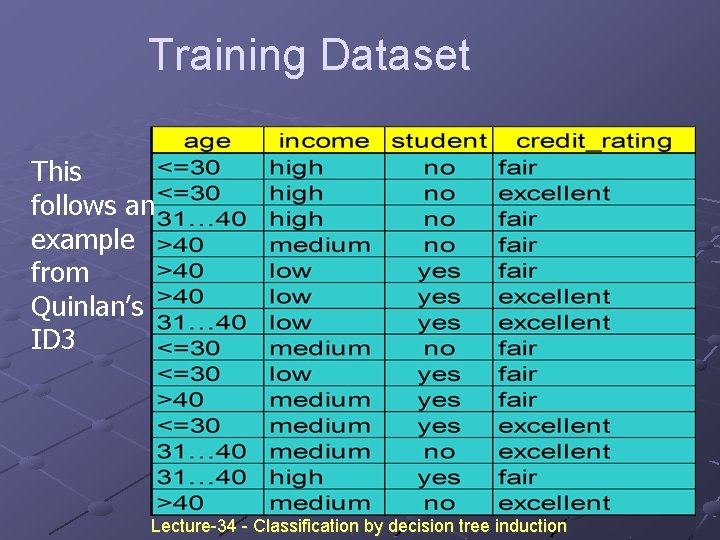
Training Dataset This follows an example from Quinlan’s ID 3 Lecture-34 - Classification by decision tree induction

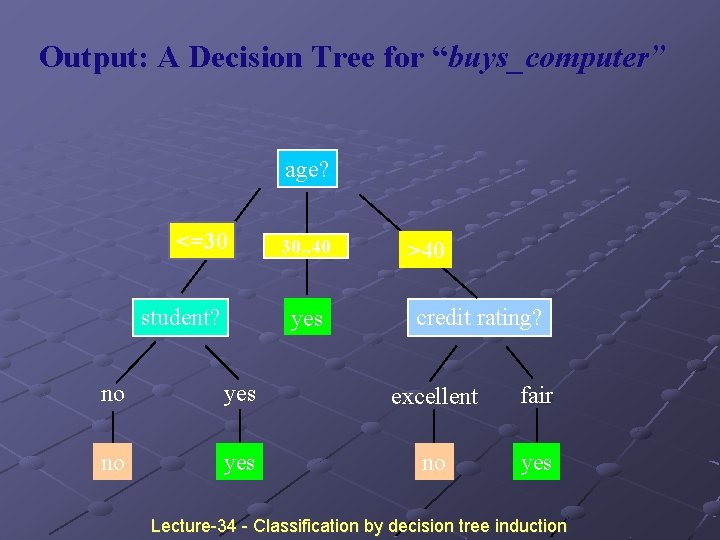
Output: A Decision Tree for “buys_computer” age? <=30 student? overcast 30. . 40 yes >40 credit rating? no yes excellent fair no yes Lecture-34 - Classification by decision tree induction

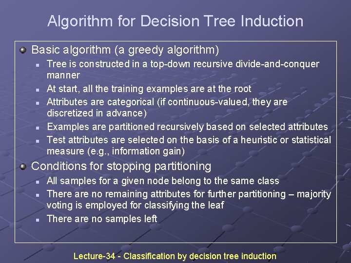
Algorithm for Decision Tree Induction Basic algorithm (a greedy algorithm) n n n Tree is constructed in a top-down recursive divide-and-conquer manner At start, all the training examples are at the root Attributes are categorical (if continuous-valued, they are discretized in advance) Examples are partitioned recursively based on selected attributes Test attributes are selected on the basis of a heuristic or statistical measure (e. g. , information gain) Conditions for stopping partitioning n n n All samples for a given node belong to the same class There are no remaining attributes for further partitioning – majority voting is employed for classifying the leaf There are no samples left Lecture-34 - Classification by decision tree induction

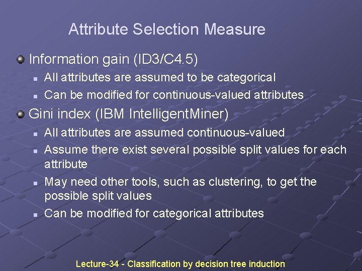
Attribute Selection Measure Information gain (ID 3/C 4. 5) n n All attributes are assumed to be categorical Can be modified for continuous-valued attributes Gini index (IBM Intelligent. Miner) n n All attributes are assumed continuous-valued Assume there exist several possible split values for each attribute May need other tools, such as clustering, to get the possible split values Can be modified for categorical attributes Lecture-34 - Classification by decision tree induction

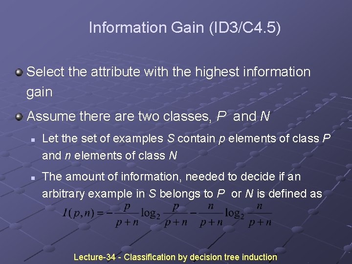
Information Gain (ID 3/C 4. 5) Select the attribute with the highest information gain Assume there are two classes, P and N n n Let the set of examples S contain p elements of class P and n elements of class N The amount of information, needed to decide if an arbitrary example in S belongs to P or N is defined as Lecture-34 - Classification by decision tree induction

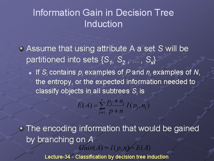
Information Gain in Decision Tree Induction Assume that using attribute A a set S will be partitioned into sets {S 1, S 2 , …, Sv} n If Si contains pi examples of P and ni examples of N, the entropy, or the expected information needed to classify objects in all subtrees Si is The encoding information that would be gained by branching on A Lecture-34 - Classification by decision tree induction

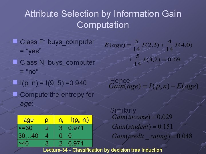
Attribute Selection by Information Gain Computation g Class P: buys_computer = “yes” g Class N: buys_computer = “no” g I(p, n) = I(9, 5) =0. 940 g Compute the entropy for age: Hence Similarly Lecture-34 - Classification by decision tree induction

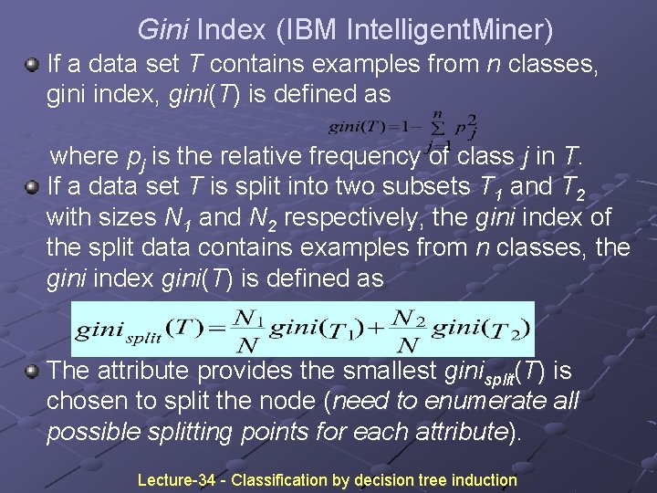
Gini Index (IBM Intelligent. Miner) If a data set T contains examples from n classes, gini index, gini(T) is defined as where pj is the relative frequency of class j in T. If a data set T is split into two subsets T 1 and T 2 with sizes N 1 and N 2 respectively, the gini index of the split data contains examples from n classes, the gini index gini(T) is defined as The attribute provides the smallest ginisplit(T) is chosen to split the node (need to enumerate all possible splitting points for each attribute). Lecture-34 - Classification by decision tree induction

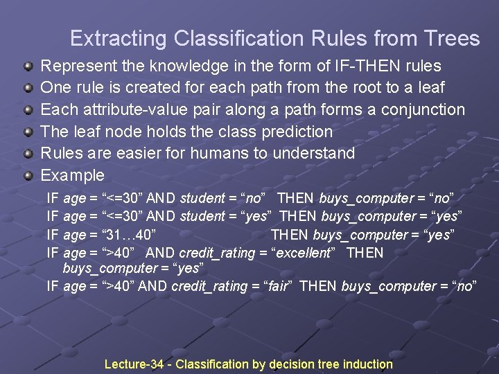
Extracting Classification Rules from Trees Represent the knowledge in the form of IF-THEN rules One rule is created for each path from the root to a leaf Each attribute-value pair along a path forms a conjunction The leaf node holds the class prediction Rules are easier for humans to understand Example IF age = “<=30” AND student = “no” THEN buys_computer = “no” IF age = “<=30” AND student = “yes” THEN buys_computer = “yes” IF age = “ 31… 40” THEN buys_computer = “yes” IF age = “>40” AND credit_rating = “excellent” THEN buys_computer = “yes” IF age = “>40” AND credit_rating = “fair” THEN buys_computer = “no” Lecture-34 - Classification by decision tree induction

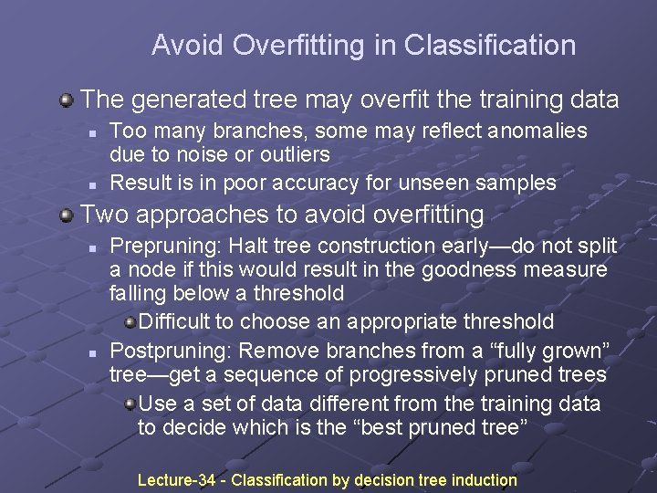
Avoid Overfitting in Classification The generated tree may overfit the training data n n Too many branches, some may reflect anomalies due to noise or outliers Result is in poor accuracy for unseen samples Two approaches to avoid overfitting n n Prepruning: Halt tree construction early—do not split a node if this would result in the goodness measure falling below a threshold Difficult to choose an appropriate threshold Postpruning: Remove branches from a “fully grown” tree—get a sequence of progressively pruned trees Use a set of data different from the training data to decide which is the “best pruned tree” Lecture-34 - Classification by decision tree induction

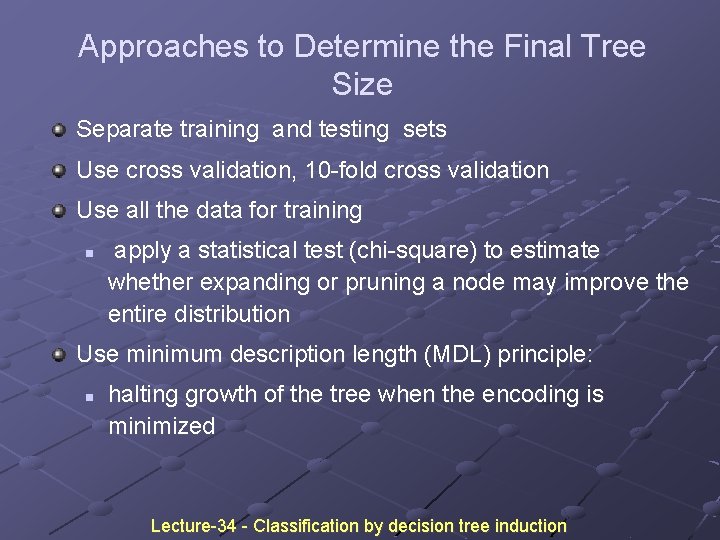
Approaches to Determine the Final Tree Size Separate training and testing sets Use cross validation, 10 -fold cross validation Use all the data for training n apply a statistical test (chi-square) to estimate whether expanding or pruning a node may improve the entire distribution Use minimum description length (MDL) principle: n halting growth of the tree when the encoding is minimized Lecture-34 - Classification by decision tree induction

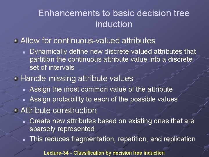
Enhancements to basic decision tree induction Allow for continuous-valued attributes n Dynamically define new discrete-valued attributes that partition the continuous attribute value into a discrete set of intervals Handle missing attribute values n n Assign the most common value of the attribute Assign probability to each of the possible values Attribute construction n n Create new attributes based on existing ones that are sparsely represented This reduces fragmentation, repetition, and replication Lecture-34 - Classification by decision tree induction

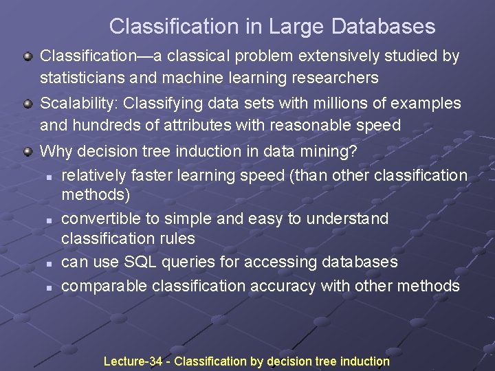
Classification in Large Databases Classification—a classical problem extensively studied by statisticians and machine learning researchers Scalability: Classifying data sets with millions of examples and hundreds of attributes with reasonable speed Why decision tree induction in data mining? n relatively faster learning speed (than other classification methods) n convertible to simple and easy to understand classification rules n can use SQL queries for accessing databases n comparable classification accuracy with other methods Lecture-34 - Classification by decision tree induction

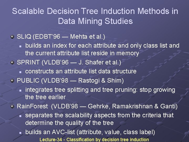
Scalable Decision Tree Induction Methods in Data Mining Studies SLIQ (EDBT’ 96 — Mehta et al. ) n builds an index for each attribute and only class list and the current attribute list reside in memory SPRINT (VLDB’ 96 — J. Shafer et al. ) n constructs an attribute list data structure PUBLIC (VLDB’ 98 — Rastogi & Shim) n integrates tree splitting and tree pruning: stop growing the tree earlier Rain. Forest (VLDB’ 98 — Gehrke, Ramakrishnan & Ganti) n separates the scalability aspects from the criteria that determine the quality of the tree n builds an AVC-list (attribute, value, class label) Lecture-34 - Classification by decision tree induction

Lecture-35 Bayesian Classification

Bayesian Classification Statical classifiers Based on Baye’s theorem Naïve Bayesian classification Class conditional independence Bayesian belief netwoks Lecture-35 - Bayesian Classification

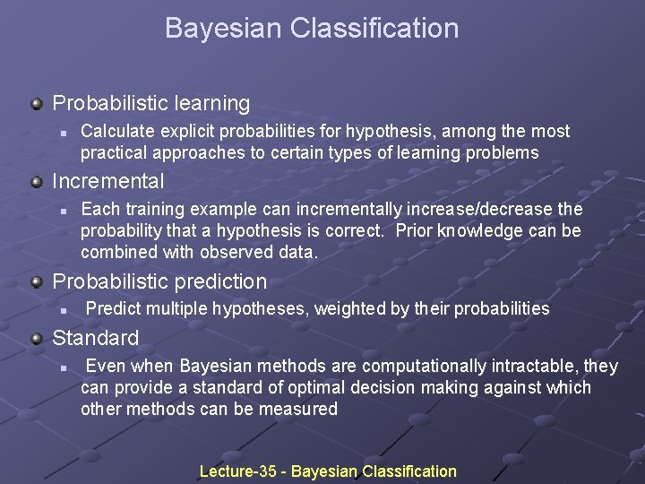
Bayesian Classification Probabilistic learning n Calculate explicit probabilities for hypothesis, among the most practical approaches to certain types of learning problems Incremental n Each training example can incrementally increase/decrease the probability that a hypothesis is correct. Prior knowledge can be combined with observed data. Probabilistic prediction n Predict multiple hypotheses, weighted by their probabilities Standard n Even when Bayesian methods are computationally intractable, they can provide a standard of optimal decision making against which other methods can be measured Lecture-35 - Bayesian Classification

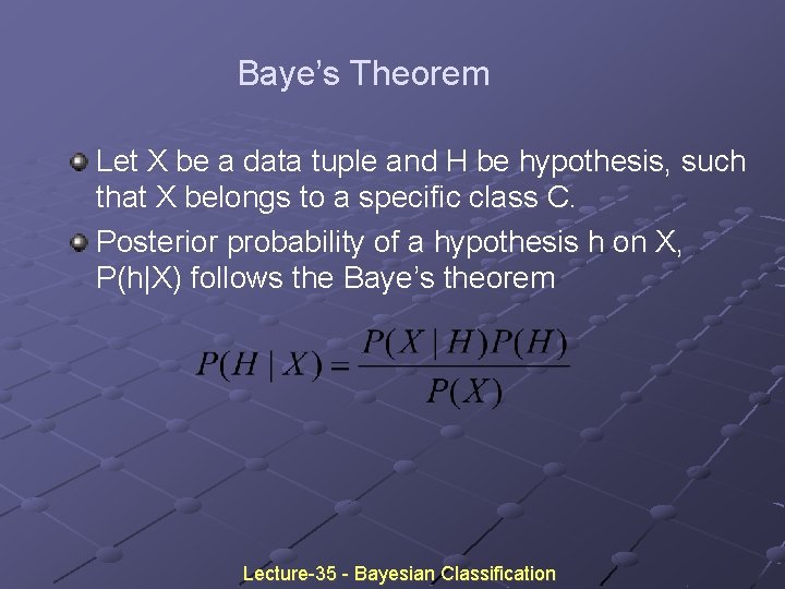
Baye’s Theorem Let X be a data tuple and H be hypothesis, such that X belongs to a specific class C. Posterior probability of a hypothesis h on X, P(h|X) follows the Baye’s theorem Lecture-35 - Bayesian Classification

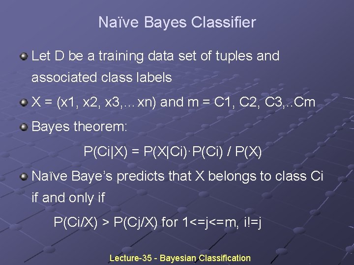
Naïve Bayes Classifier Let D be a training data set of tuples and associated class labels X = (x 1, x 2, x 3, …xn) and m = C 1, C 2, C 3, . . Cm Bayes theorem: P(Ci|X) = P(X|Ci)·P(Ci) / P(X) Naïve Baye’s predicts that X belongs to class Ci if and only if P(Ci/X) > P(Cj/X) for 1<=j<=m, i!=j Lecture-35 - Bayesian Classification

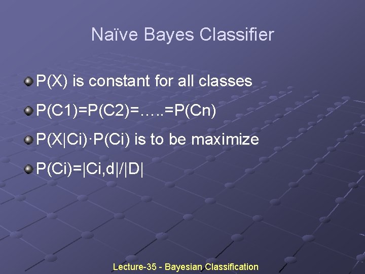
Naïve Bayes Classifier P(X) is constant for all classes P(C 1)=P(C 2)=…. . =P(Cn) P(X|Ci)·P(Ci) is to be maximize P(Ci)=|Ci, d|/|D| Lecture-35 - Bayesian Classification

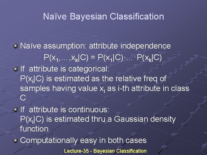
Naïve Bayesian Classification Naïve assumption: attribute independence P(x 1, …, xk|C) = P(x 1|C)·…·P(xk|C) If attribute is categorical: P(xi|C) is estimated as the relative freq of samples having value xi as i-th attribute in class C If attribute is continuous: P(xi|C) is estimated thru a Gaussian density function Computationally easy in both cases Lecture-35 - Bayesian Classification

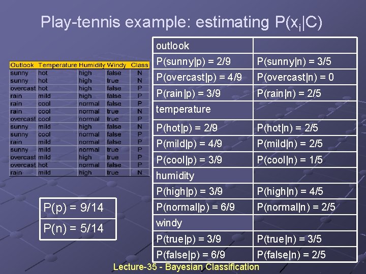
Play-tennis example: estimating P(xi|C) outlook P(sunny|p) = 2/9 P(sunny|n) = 3/5 P(overcast|p) = 4/9 P(overcast|n) = 0 P(rain|p) = 3/9 P(rain|n) = 2/5 temperature P(hot|p) = 2/9 P(hot|n) = 2/5 P(mild|p) = 4/9 P(mild|n) = 2/5 P(cool|p) = 3/9 P(cool|n) = 1/5 humidity P(high|p) = 3/9 P(high|n) = 4/5 P(p) = 9/14 P(normal|p) = 6/9 P(normal|n) = 2/5 P(n) = 5/14 windy P(true|p) = 3/9 P(true|n) = 3/5 P(false|p) = 6/9 P(false|n) = 2/5 Lecture-35 - Bayesian Classification

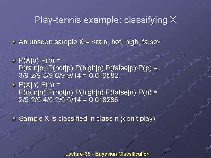
Play-tennis example: classifying X An unseen sample X = <rain, hot, high, false> P(X|p)·P(p) = P(rain|p)·P(hot|p)·P(high|p)·P(false|p)·P(p) = 3/9· 2/9· 3/9· 6/9· 9/14 = 0. 010582 P(X|n)·P(n) = P(rain|n)·P(hot|n)·P(high|n)·P(false|n)·P(n) = 2/5· 4/5· 2/5· 5/14 = 0. 018286 Sample X is classified in class n (don’t play) Lecture-35 - Bayesian Classification

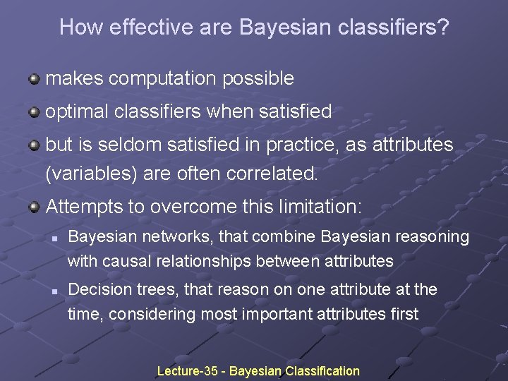
How effective are Bayesian classifiers? makes computation possible optimal classifiers when satisfied but is seldom satisfied in practice, as attributes (variables) are often correlated. Attempts to overcome this limitation: n n Bayesian networks, that combine Bayesian reasoning with causal relationships between attributes Decision trees, that reason on one attribute at the time, considering most important attributes first Lecture-35 - Bayesian Classification

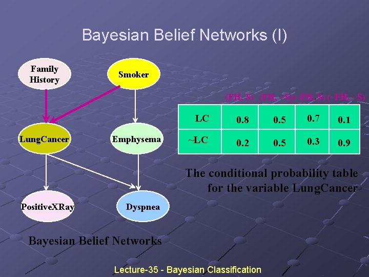
Bayesian Belief Networks (I) Family History Smoker (FH, S) (FH, ~S)(~FH, S) (~FH, ~S) Lung. Cancer Emphysema LC 0. 8 0. 5 0. 7 0. 1 ~LC 0. 2 0. 5 0. 3 0. 9 The conditional probability table for the variable Lung. Cancer Positive. XRay Dyspnea Bayesian Belief Networks Lecture-35 - Bayesian Classification

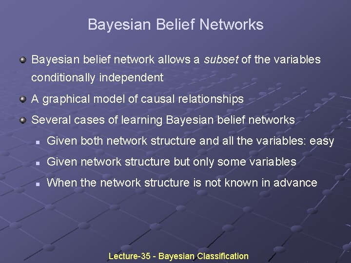
Bayesian Belief Networks Bayesian belief network allows a subset of the variables conditionally independent A graphical model of causal relationships Several cases of learning Bayesian belief networks n Given both network structure and all the variables: easy n Given network structure but only some variables n When the network structure is not known in advance Lecture-35 - Bayesian Classification

Lecture-36 Classification by Backpropagation

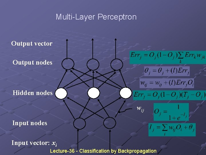
Classification by Backpropagation Neural network learning algorithm Psychologists and Neurobiologists Neural network – set of connected input/output units in which each connection has a weight associated with it. Lecture-36 - Classification by Backpropagation

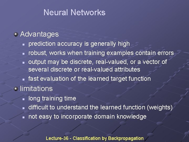
Neural Networks Advantages n n prediction accuracy is generally high robust, works when training examples contain errors output may be discrete, real-valued, or a vector of several discrete or real-valued attributes fast evaluation of the learned target function limitations n n n long training time difficult to understand the learned function (weights) not easy to incorporate domain knowledge Lecture-36 - Classification by Backpropagation

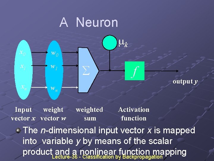
x 0 w 0 x 1 w 1 xn A Neuron - mk å f wn Input weight vector x vector w weighted sum output y Activation function The n-dimensional input vector x is mapped into variable y by means of the scalar product. Lecture-36 and a -nonlinear function mapping Classification by Backpropagation

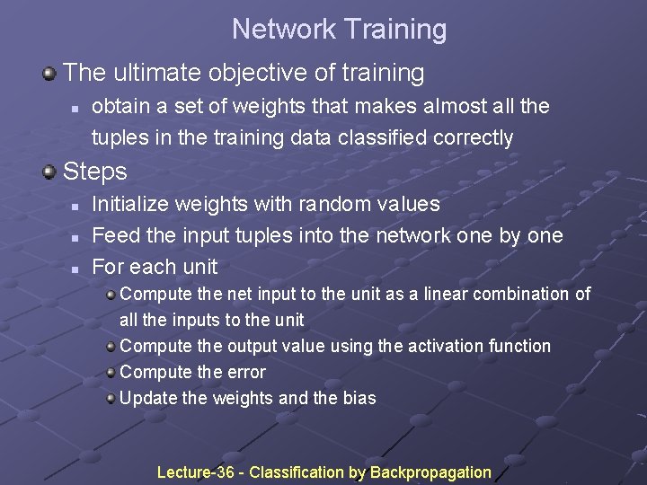
Network Training The ultimate objective of training n obtain a set of weights that makes almost all the tuples in the training data classified correctly Steps n n n Initialize weights with random values Feed the input tuples into the network one by one For each unit Compute the net input to the unit as a linear combination of all the inputs to the unit Compute the output value using the activation function Compute the error Update the weights and the bias Lecture-36 - Classification by Backpropagation

Multi-Layer Perceptron Output vector Output nodes Hidden nodes wij Input nodes Input vector: xi Lecture-36 - Classification by Backpropagation

Lecture-37 Classification based on concepts from association rule mining

Association-Based Classification Several methods for association-based classification n ARCS: Quantitative association mining and clustering of association rules (Lent et al’ 97) It beats C 4. 5 in (mainly) scalability and also accuracy n Associative classification: (Liu et al’ 98) It mines high support and high confidence rules in the form of “cond_set => y”, where y is a class label Lecture-37 - Classification based on concepts from association rule mining

Association-Based Classification n CAEP (Classification by aggregating emerging patterns) (Dong et al’ 99) Emerging patterns (EPs): the itemsets whose support increases significantly from one class to another Mine Eps based on minimum support and growth rate Lecture-37 - Classification based on concepts from association rule mining

Lecture-38 Other Classification Methods

Other Classification Methods k-nearest neighbor classifier case-based reasoning Genetic algorithm Rough set approach Fuzzy set approaches Lecture-38 - Other Classification Methods

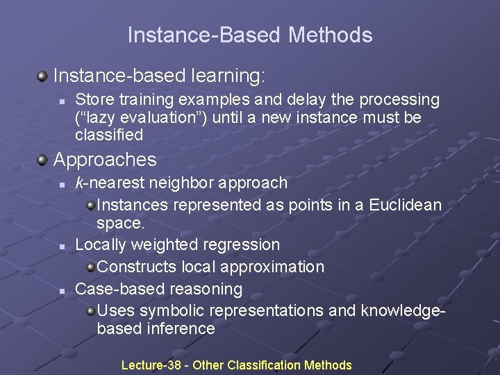
Instance-Based Methods Instance-based learning: n Store training examples and delay the processing (“lazy evaluation”) until a new instance must be classified Approaches n n n k-nearest neighbor approach Instances represented as points in a Euclidean space. Locally weighted regression Constructs local approximation Case-based reasoning Uses symbolic representations and knowledgebased inference Lecture-38 - Other Classification Methods

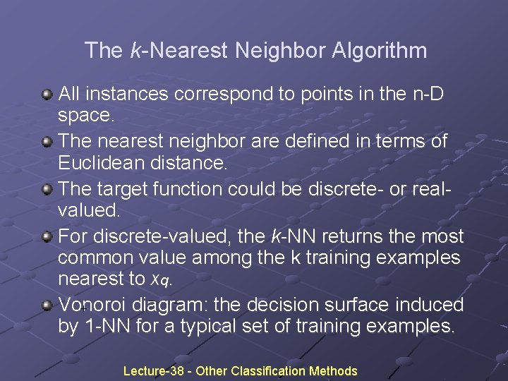
The k-Nearest Neighbor Algorithm All instances correspond to points in the n-D space. The nearest neighbor are defined in terms of Euclidean distance. The target function could be discrete- or realvalued. For discrete-valued, the k-NN returns the most common value among the k training examples nearest to xq. _ _ Vonoroi diagram: the decision surface induced + by 1 -NN for a typical set of training examples. Lecture-38 - Other Classification Methods

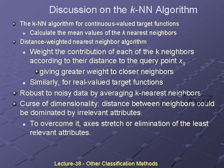
Discussion on the k-NN Algorithm The k-NN algorithm for continuous-valued target functions n Calculate the mean values of the k nearest neighbors Distance-weighted nearest neighbor algorithm Weight the contribution of each of the k neighbors according to their distance to the query point xq giving greater weight to closer neighbors n Similarly, for real-valued target functions Robust to noisy data by averaging k-nearest neighbors Curse of dimensionality: distance between neighbors could be dominated by irrelevant attributes. n To overcome it, axes stretch or elimination of the least relevant attributes. n Lecture-38 - Other Classification Methods

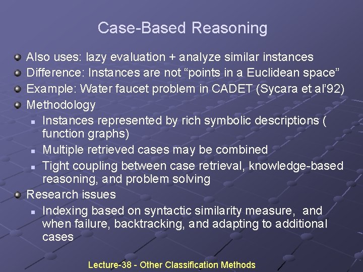
Case-Based Reasoning Also uses: lazy evaluation + analyze similar instances Difference: Instances are not “points in a Euclidean space” Example: Water faucet problem in CADET (Sycara et al’ 92) Methodology n Instances represented by rich symbolic descriptions ( function graphs) n Multiple retrieved cases may be combined n Tight coupling between case retrieval, knowledge-based reasoning, and problem solving Research issues n Indexing based on syntactic similarity measure, and when failure, backtracking, and adapting to additional cases Lecture-38 - Other Classification Methods

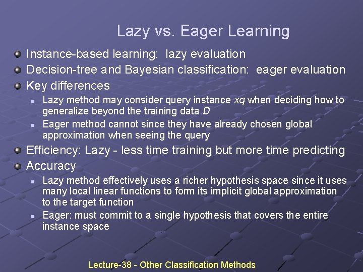
Lazy vs. Eager Learning Instance-based learning: lazy evaluation Decision-tree and Bayesian classification: eager evaluation Key differences n n Lazy method may consider query instance xq when deciding how to generalize beyond the training data D Eager method cannot since they have already chosen global approximation when seeing the query Efficiency: Lazy - less time training but more time predicting Accuracy n n Lazy method effectively uses a richer hypothesis space since it uses many local linear functions to form its implicit global approximation to the target function Eager: must commit to a single hypothesis that covers the entire instance space Lecture-38 - Other Classification Methods

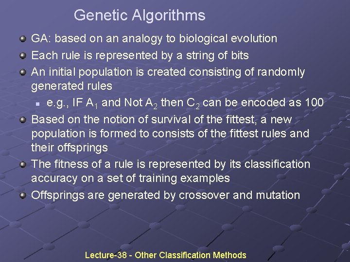
Genetic Algorithms GA: based on an analogy to biological evolution Each rule is represented by a string of bits An initial population is created consisting of randomly generated rules n e. g. , IF A 1 and Not A 2 then C 2 can be encoded as 100 Based on the notion of survival of the fittest, a new population is formed to consists of the fittest rules and their offsprings The fitness of a rule is represented by its classification accuracy on a set of training examples Offsprings are generated by crossover and mutation Lecture-38 - Other Classification Methods

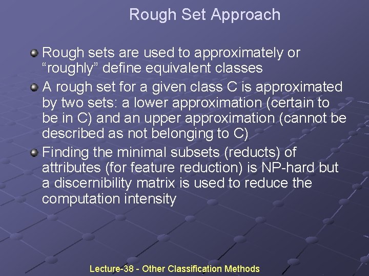
Rough Set Approach Rough sets are used to approximately or “roughly” define equivalent classes A rough set for a given class C is approximated by two sets: a lower approximation (certain to be in C) and an upper approximation (cannot be described as not belonging to C) Finding the minimal subsets (reducts) of attributes (for feature reduction) is NP-hard but a discernibility matrix is used to reduce the computation intensity Lecture-38 - Other Classification Methods

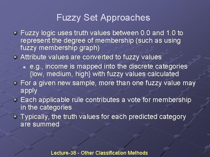
Fuzzy Set Approaches Fuzzy logic uses truth values between 0. 0 and 1. 0 to represent the degree of membership (such as using fuzzy membership graph) Attribute values are converted to fuzzy values n e. g. , income is mapped into the discrete categories {low, medium, high} with fuzzy values calculated For a given new sample, more than one fuzzy value may apply Each applicable rule contributes a vote for membership in the categories Typically, the truth values for each predicted category are summed Lecture-38 - Other Classification Methods

Lecture-39 Prediction

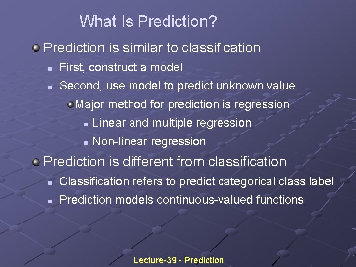
What Is Prediction? Prediction is similar to classification n First, construct a model n Second, use model to predict unknown value Major method for prediction is regression n Linear and multiple regression n Non-linear regression Prediction is different from classification n Classification refers to predict categorical class label n Prediction models continuous-valued functions Lecture-39 - Prediction

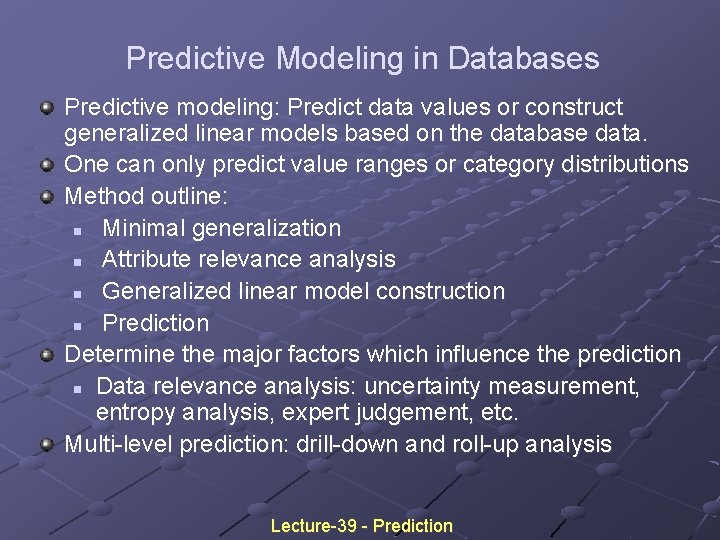
Predictive Modeling in Databases Predictive modeling: Predict data values or construct generalized linear models based on the database data. One can only predict value ranges or category distributions Method outline: n Minimal generalization n Attribute relevance analysis n Generalized linear model construction n Prediction Determine the major factors which influence the prediction n Data relevance analysis: uncertainty measurement, entropy analysis, expert judgement, etc. Multi-level prediction: drill-down and roll-up analysis Lecture-39 - Prediction

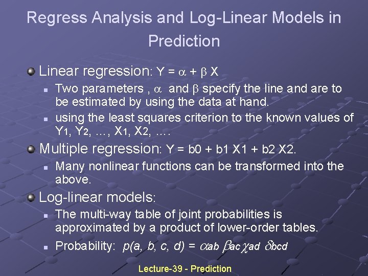
Regress Analysis and Log-Linear Models in Prediction Linear regression: Y = + X Two parameters , and specify the line and are to be estimated by using the data at hand. n using the least squares criterion to the known values of Y 1, Y 2, …, X 1, X 2, …. Multiple regression: Y = b 0 + b 1 X 1 + b 2 X 2. n Many nonlinear functions can be transformed into the above. Log-linear models: n The multi-way table of joint probabilities is approximated by a product of lower-order tables. n Probability: p(a, b, c, d) = ab ac ad bcd n Lecture-39 - Prediction

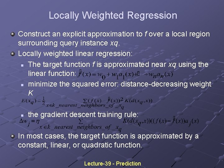
Locally Weighted Regression Construct an explicit approximation to f over a local region surrounding query instance xq. Locally weighted linear regression: n The target function f is approximated near xq using the linear function: n minimize the squared error: distance-decreasing weight K n the gradient descent training rule: In most cases, the target function is approximated by a constant, linear, or quadratic function. Lecture-39 - Prediction

Lecture-40 Classification accuracy

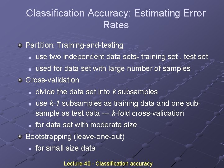
Classification Accuracy: Estimating Error Rates Partition: Training-and-testing n use two independent data sets- training set , test set n used for data set with large number of samples Cross-validation n divide the data set into k subsamples use k-1 subsamples as training data and one subsample as test data --- k-fold cross-validation for data set with moderate size Bootstrapping (leave-one-out) n for small size data Lecture-40 - Classification accuracy

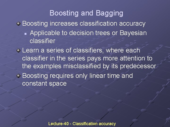
Boosting and Bagging Boosting increases classification accuracy n Applicable to decision trees or Bayesian classifier Learn a series of classifiers, where each classifier in the series pays more attention to the examples misclassified by its predecessor Boosting requires only linear time and constant space Lecture-40 - Classification accuracy

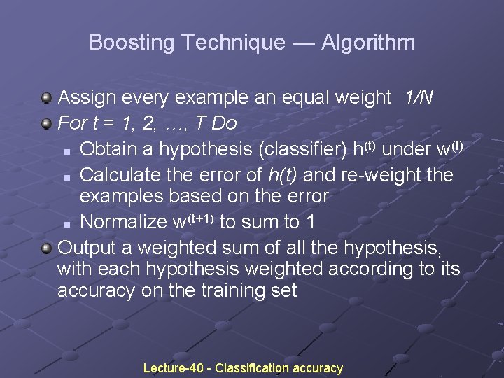
Boosting Technique — Algorithm Assign every example an equal weight 1/N For t = 1, 2, …, T Do (t) under w(t) n Obtain a hypothesis (classifier) h n Calculate the error of h(t) and re-weight the examples based on the error (t+1) to sum to 1 n Normalize w Output a weighted sum of all the hypothesis, with each hypothesis weighted according to its accuracy on the training set Lecture-40 - Classification accuracy