Unit3 objectives 1 Introduction to trees 2 Representation

Unit-3 objectives 1. Introduction to trees. 2. Representation of trees. 3. Binary tree ADT. 4. Properties of trees. 5. Binary tree representations-array and linked representations. 6. Binary tree traversals. 7. Threaded binary tree. 8. MAX priority Queue ADT-implementation. 9. Max Heap- Definition, insertion into and deletion from a Max Heap. 10. Graphs- Introduction, definition, terminalogy 11. Graph ADT. 12. Graph representations-Adjacency matrix, Adjacency lists 13. Graph traversals-BFS, DFS

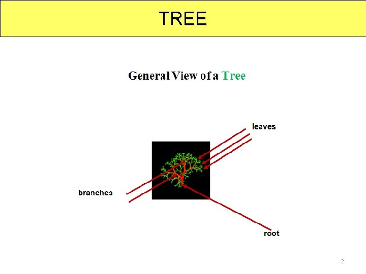
TREE 2

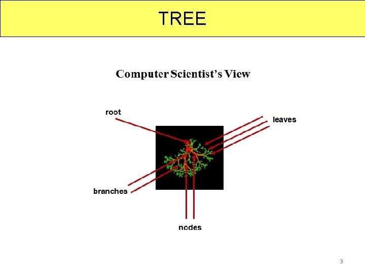
TREE 3

Linear Lists And Trees • Linear lists are useful for serially ordered data. – (e 0, e 1, e 2, …, en-1) – Days of week. – Months in a year. – Students in this class. • Trees are useful for hierarchically ordered data. – Employees of a corporation. • President, vice presidents, managers, and so on.

Hierarchical Data And Trees • The element at the top of the hierarchy is the root. • Elements next in the hierarchy are the children of the root. • Elements next in the hierarchy are the grandchildren of the root, and so on. • Elements that have no children are leaves.

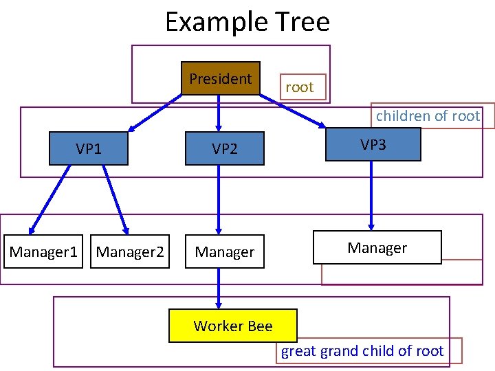
Example Tree President root children of root VP 1 Manager 2 VP 2 Manager VP 3 Manager grand children of root Worker Bee great grand child of root

TREE Definition: • A tree is a finite of one or more nodes such that • There is specially designated node called root. • The remaining node are partitioned in to n>=0 disjoint sets T 1, T 2, T 3…. Tn, where each of these sets in a tree. • T 1, T 2, T 3…. Tn, are called the subtrees of the root. t

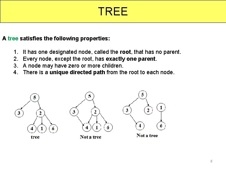
TREE A tree satisfies the following properties: 1. 2. 3. 4. It has one designated node, called the root, that has no parent. Every node, except the root, has exactly one parent. A node may have zero or more children. There is a unique directed path from the root to each node. 8

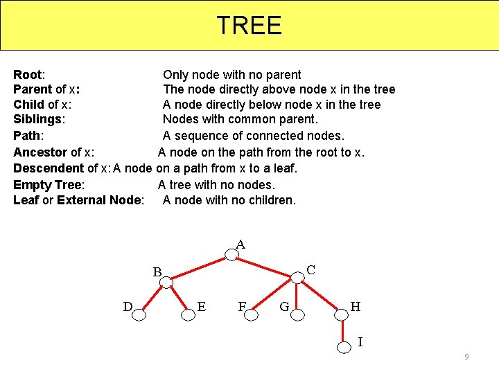
TREE Root: Only node with no parent Parent of x: The node directly above node x in the tree Child of x: A node directly below node x in the tree Siblings: Nodes with common parent. Path: A sequence of connected nodes. Ancestor of x: A node on the path from the root to x. Descendent of x: A node on a path from x to a leaf. Empty Tree: A tree with no nodes. Leaf or External Node: A node with no children. A C B D E F G H I 9

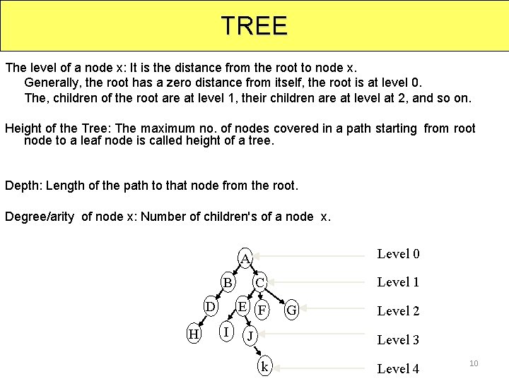
TREE The level of a node x: It is the distance from the root to node x. Generally, the root has a zero distance from itself, the root is at level 0. The, children of the root are at level 1, their children are at level at 2, and so on. Height of the Tree: The maximum no. of nodes covered in a path starting from root node to a leaf node is called height of a tree. Depth: Length of the path to that node from the root. Degree/arity of node x: Number of children's of a node x. Level 0 A B D H E F I Level 1 C J G Level 2 Level 3 k Level 4 10

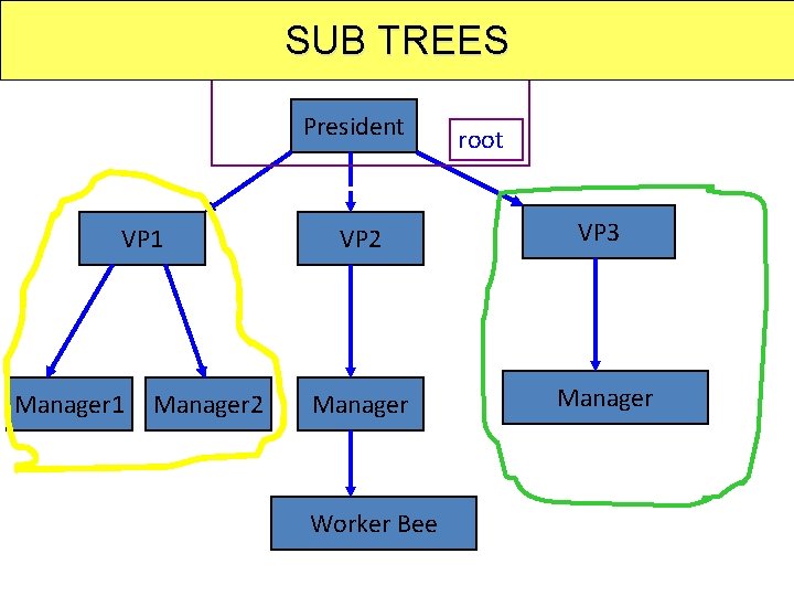
SUB TREES President VP 1 Manager 2 root VP 2 VP 3 Manager Worker Bee

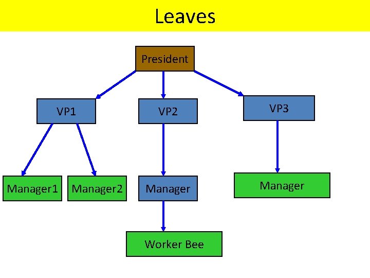
Leaves President VP 1 Manager 2 VP 3 Manager Worker Bee

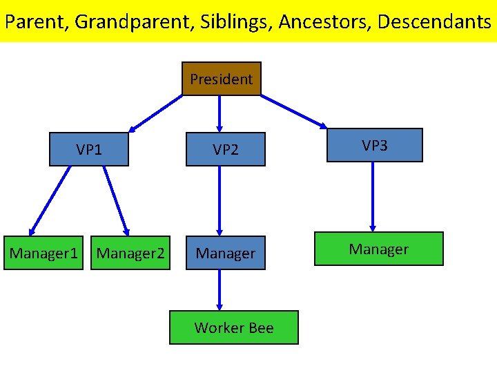
Parent, Grandparent, Siblings, Ancestors, Descendants President VP 1 Manager 2 VP 3 Manager Worker Bee

Caution • Some texts start level numbers at 0 rather than at 1. • Root is at level 0. • Its children are at level 1. • The grand children of the root are at level 2. • And so on. • We shall number levels with the root at level 1.

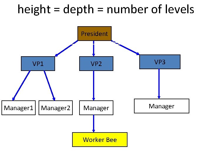
height = depth = number of levels President Level 1 Level 2 VP 1 Manager 2 VP 3 Manager Level 3 Worker Bee Level 4

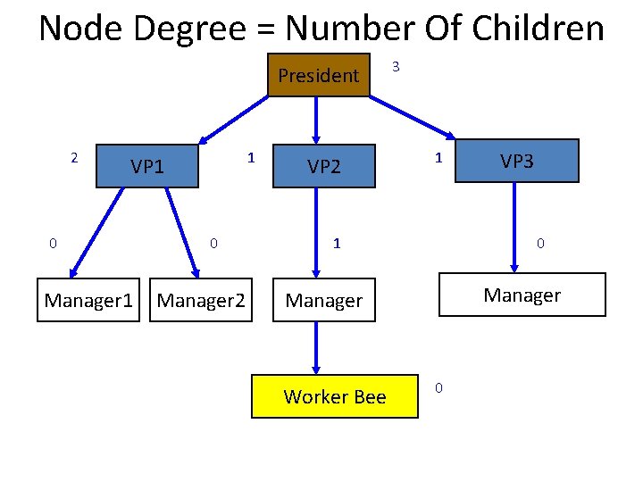
Node Degree = Number Of Children President 2 1 VP 1 0 Manager 2 VP 2 3 1 1 0 Manager Worker Bee VP 3 0

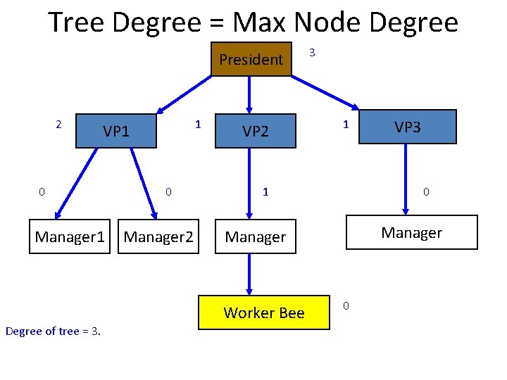
Tree Degree = Max Node Degree President 2 1 VP 1 0 Manager 2 VP 2 1 1 VP 3 0 Manager Worker Bee Degree of tree = 3. 3 0

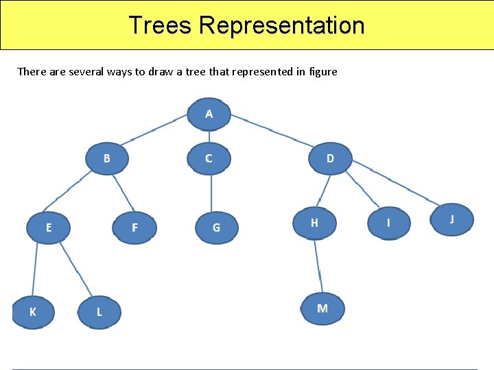
Trees Representation There are several ways to draw a tree that represented in figure

Trees Representation There are three ways to represent a tree 1. 2. 3. List representation Left child-Right sibling representation Representation as a Degree-Two tree 1. List representation: The tree shown above can be written as the list ( A ( B ( E ( K , L ) , F) , C ( G ) , D ( H ( M ) , I , J ) ) ) The information in the root node comes first, followed by a list of sub tress of that node.

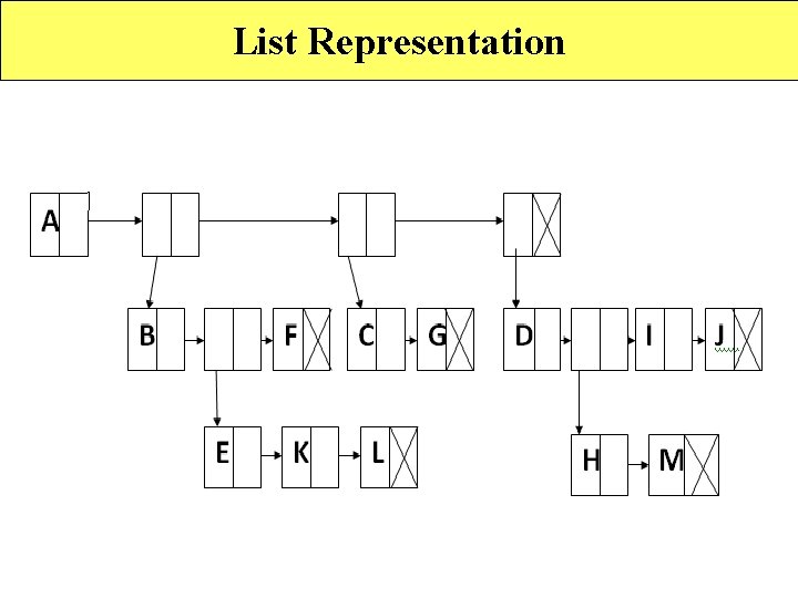
List Representation

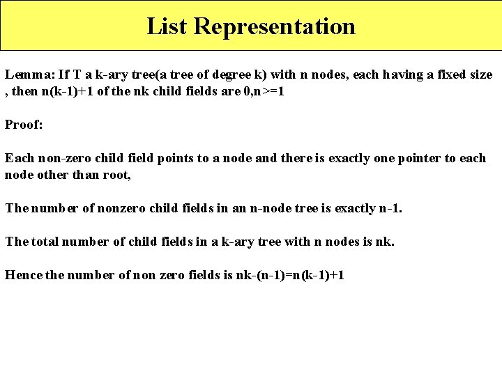
List Representation Lemma: If T a k-ary tree(a tree of degree k) with n nodes, each having a fixed size , then n(k-1)+1 of the nk child fields are 0, n>=1 Proof: Each non-zero child field points to a node and there is exactly one pointer to each node other than root, The number of nonzero child fields in an n-node tree is exactly n-1. The total number of child fields in a k-ary tree with n nodes is nk. Hence the number of non zero fields is nk-(n-1)=n(k-1)+1

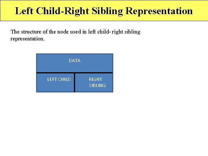
Left Child-Right Sibling Representation The structure of the node used in left child- right sibling representation. DATA LEFT CHILD RIGHT SIBLING

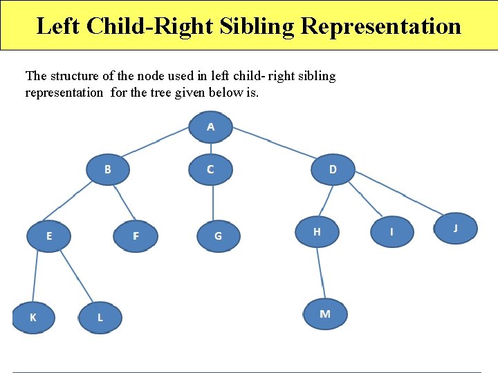
Left Child-Right Sibling Representation The structure of the node used in left child- right sibling representation for the tree given below is.

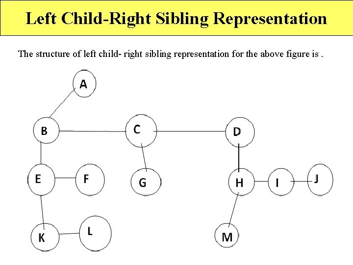
Left Child-Right Sibling Representation The structure of left child- right sibling representation for the above figure is.

Representation as a Degree-Two tree 1. To obtain the degree-two tree representation of a tree we simply rotate the right sibling pointers in a left child- right sibling tree clockwise by 45 degrees 2. We refer to the two children of a node as the left and right children. 3. Notice that the right of the root node is empty 4. Left child –right child trees are also known as binary trees.

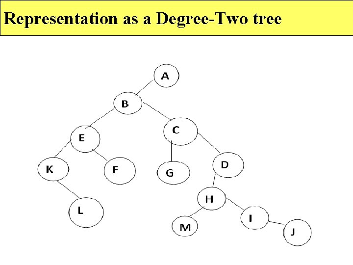
Representation as a Degree-Two tree

TREE APPLICATIONS Trees are very important data structures in computing. They are suitable for: • Hierarchical structure representation, e. g. , • File directory. • Organizational structure of an institution. • Class inheritance tree. • Problem representation, e. g. , • Expression tree. • Decision tree. • Efficient algorithmic solutions, e. g. , • Search trees. • Efficient priority queues via heaps. 27

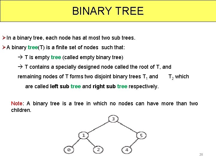
BINARY TREE ØIn a binary tree, each node has at most two sub trees. ØA binary tree(T) is a finite set of nodes such that: T is empty tree (called empty binary tree) T contains a specially designed node called the root of T, and remaining nodes of T forms two disjoint binary trees T 1 and T 2 which are called left sub tree and right sub tree respectively. Note: A binary tree is a tree in which no nodes can have more than two children. 28

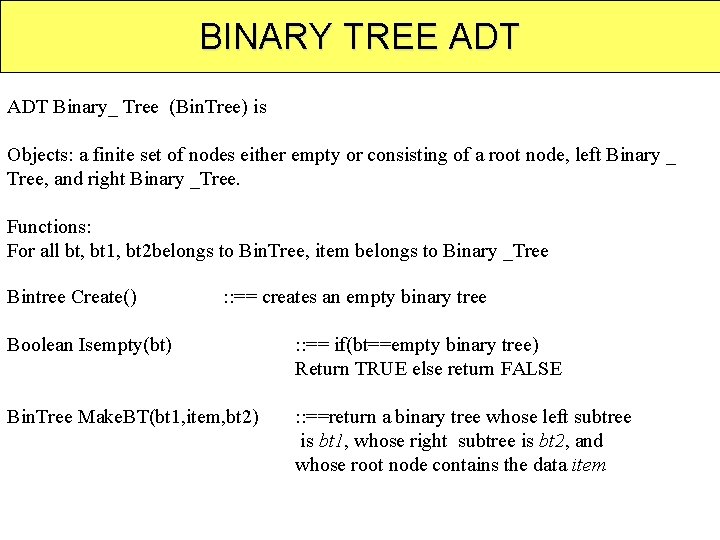
BINARY TREE ADT Binary_ Tree (Bin. Tree) is Objects: a finite set of nodes either empty or consisting of a root node, left Binary _ Tree, and right Binary _Tree. Functions: For all bt, bt 1, bt 2 belongs to Bin. Tree, item belongs to Binary _Tree Bintree Create() : : == creates an empty binary tree Boolean Isempty(bt) : : == if(bt==empty binary tree) Return TRUE else return FALSE Bin. Tree Make. BT(bt 1, item, bt 2) : : ==return a binary tree whose left subtree is bt 1, whose right subtree is bt 2, and whose root node contains the data item

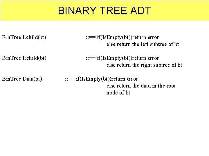
BINARY TREE ADT Bin. Tree Lchild(bt) : : == if(Is. Empty(bt))return error else return the left subtree of bt Bin. Tree Rchild(bt) : : == if(Is. Empty(bt))return error else return the right subtree of bt Bin. Tree Data(bt) : : == if(Is. Empty(bt))return error else return the data in the root node of bt

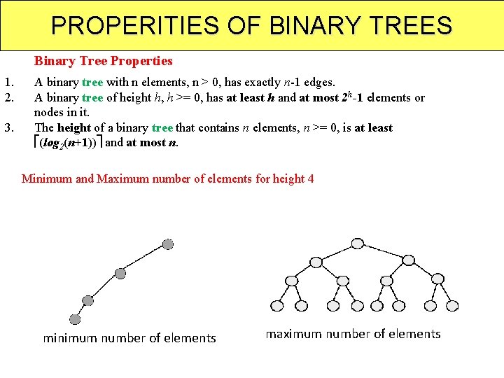
PROPERITIES OF BINARY TREES Binary Tree Properties 1. 2. 3. A binary tree with n elements, n > 0, has exactly n-1 edges. A binary tree of height h, h >= 0, has at least h and at most 2 h-1 elements or nodes in it. The height of a binary tree that contains n elements, n >= 0, is at least (log 2(n+1)) and at most n. Minimum and Maximum number of elements for height 4 minimum number of elements maximum number of elements

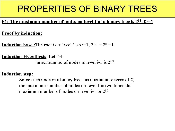
PROPERITIES OF BINARY TREES P 1: The maximum number of nodes on level I of a binary tree is 2 i-1, i>=1 Proof by induction: Induction base : The root is at level 1 so i=1, 21 -1 = 20 =1 Induction Hypothesis: Let i>1 maximum no of nodes at level i-1 is 2 i-2 Induction step: Since each node in a binary tree has maximum degree of 2, the maximum number of nodes on level I is two times the maximum number of nodes on level i-1 or 2 i-1

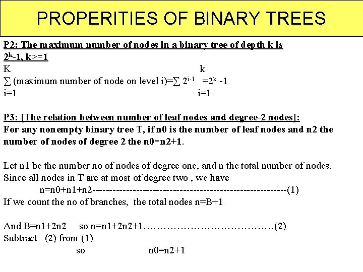
PROPERITIES OF BINARY TREES P 2: The maximum number of nodes in a binary tree of depth k is 2 k-1, k>=1 K k ∑ (maximum number of node on level i)=∑ 2 i-1 =2 k -1 i=1 P 3: [The relation between number of leaf nodes and degree-2 nodes]: For any nonempty binary tree T, if n 0 is the number of leaf nodes and n 2 the number of nodes of degree 2 the n 0=n 2+1. Let n 1 be the number no of nodes of degree one, and n the total number of nodes. Since all nodes in T are at most of degree two , we have n=n 0+n 1+n 2 -----------------------------(1) If we count the no of branches, the total nodes n=B+1 And B=n 1+2 n 2 so n=n 1+2 n 2+1…………………(2) Subtract (2) from (1) so n 0=n 2+1

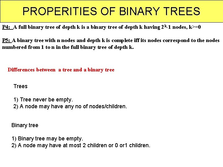
PROPERITIES OF BINARY TREES P 4: A full binary tree of depth k is a binary tree of depth k having 2 k-1 nodes, k>=0 P 5: A binary tree with n nodes and depth k is complete iff its nodes correspond to the nodes numbered from 1 to n in the full binary tree of depth k. Differences between a tree and a binary tree Trees 1) Tree never be empty. 2) A node may have any no of nodes/children. Binary tree 1) Binary tree may be empty. 2) A node may have at most 2 children or 0 or 1 children.

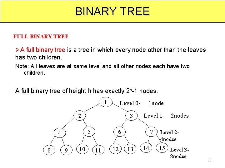
BINARY TREE FULL BINARY TREE ØA full binary tree is a tree in which every node other than the leaves has two children. Note: All leaves are at same level and all other nodes each have two children. A full binary tree of height h has exactly 2 h-1 nodes. 1 Level 0 - 1 node 2 5 4 8 3 9 10 Level 1 - 2 nodes 6 11 12 7 13 14 Level 2 - 4 nodes 15 Level 38 nodes 35

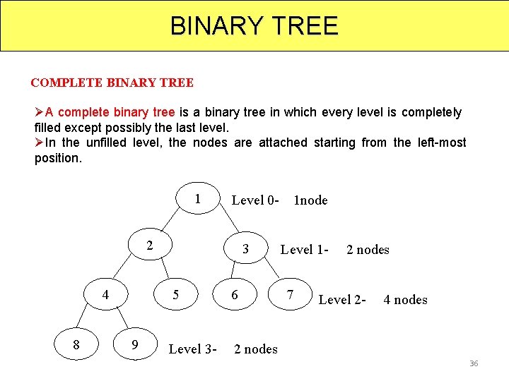
BINARY TREE COMPLETE BINARY TREE ØA complete binary tree is a binary tree in which every level is completely filled except possibly the last level. ØIn the unfilled level, the nodes are attached starting from the left-most position. 1 Level 0 - 1 node 2 4 8 3 5 9 6 Level 1 - 2 nodes 7 Level 2 - 4 nodes Level 3 - 2 nodes 36

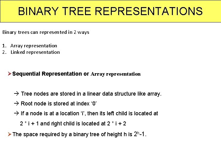
BINARY TREE REPRESENTATIONS Binary trees can represented in 2 ways 1. Array representation 2. Linked representation ØSequential Representation or Array representation Tree nodes are stored in a linear data structure like array. Root node is stored at index ‘ 0’ If a node is at a location ‘i’, then its left child is located at 2 * i + 1 and right child is located at 2 * i + 2 ØThe space required by a binary tree of height h is 2 h-1.

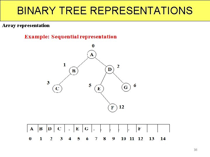
BINARY TREE REPRESENTATIONS Array representation 38

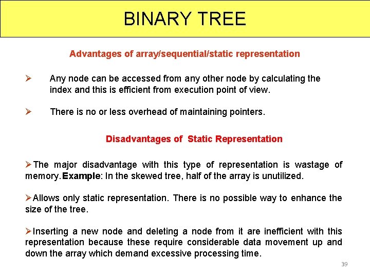
BINARY TREE Advantages of array/sequential/static representation Ø Any node can be accessed from any other node by calculating the index and this is efficient from execution point of view. Ø There is no or less overhead of maintaining pointers. Disadvantages of Static Representation ØThe major disadvantage with this type of representation is wastage of memory. Example: In the skewed tree, half of the array is unutilized. ØAllows only static representation. There is no possible way to enhance the size of the tree. ØInserting a new node and deleting a node from it are inefficient with this representation because these require considerable data movement up and down the array which demand excessive processing time. 39

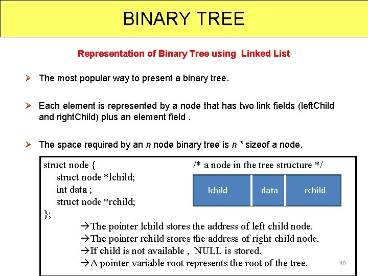
BINARY TREE Representation of Binary Tree using Linked List Ø The most popular way to present a binary tree. Ø Each element is represented by a node that has two link fields (left. Child and right. Child) plus an element field. Ø The space required by an n node binary tree is n * sizeof a node. struct node { /* a node in the tree structure */ struct node *lchild; int data ; lchild data rchild struct node *rchild; }; The pointer lchild stores the address of left child node. The pointer rchild stores the address of right child node. If child is not available , NULL is stored. A pointer variable root represents the root of the tree. 40

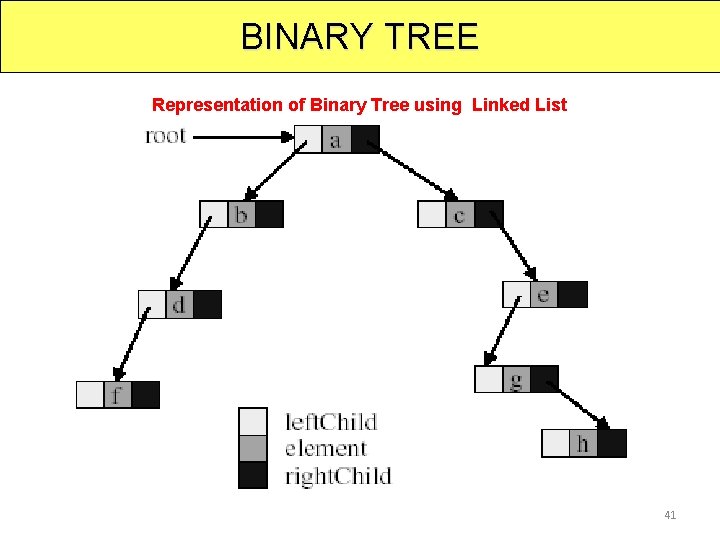
BINARY TREE Representation of Binary Tree using Linked List 41

BINARY TREE Advantages of linked representation ØThis representation is superior to the array representation as there is no wastage of memory. ØThere is no need to have prior knowledge of depth of the tree. Using dynamic memory allocation concept one can create as much memory (node) as required. ØInsertion and deletion which are the most common operations can be done without moving the other nodes. Disadvantages of linked representation Ø This representation does not provide direct access to a node. Ø It needs additional space in each node for storing the left and right subtrees 42

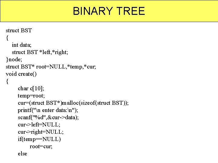
BINARY TREE struct BST { int data; struct BST *left, *right; }node; struct BST* root=NULL, *temp, *cur; void create() { char c[10]; temp=root; cur=(struct BST*)malloc(sizeof(struct BST)); printf("n enter data: n"); scanf("%d", &cur->data); cur->left=NULL; cur->right=NULL; if(temp==NULL) root=cur; else

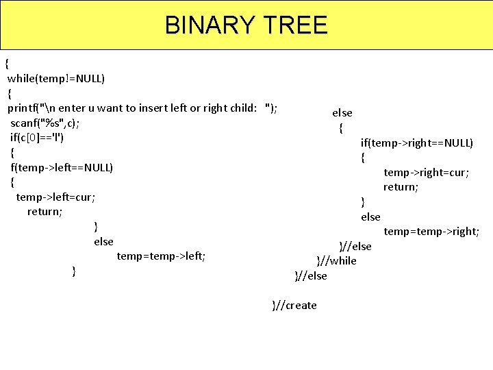
BINARY TREE { while(temp!=NULL) { printf("n enter u want to insert left or right child: "); scanf("%s", c); if(c[0]=='l') { f(temp->left==NULL) { temp->left=cur; return; } else temp=temp->left; } else { if(temp->right==NULL) { temp->right=cur; return; } else temp=temp->right; }//else }//while }//else }//create

BINARY TREE TRAVERSALS Traversal : visiting each node at least once Traversal can be done in two ways 1. Recursive traversal 2. Iterative traversal ØThere are six recursive and non recursive techniques for binary tree traversal. 1. Preorder Traversal 2. Inorder Traversal 3. Postorder Traversal 4. Converse Preorder Traversal 5. Converse Inorder Traversal 6. Converse Postorder Traversal 45

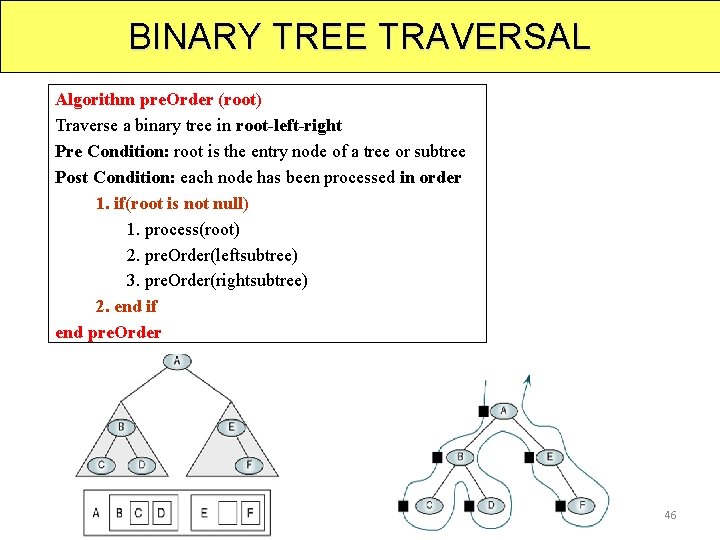
BINARY TREE TRAVERSAL Algorithm pre. Order (root) Traverse a binary tree in root-left-right Pre Condition: root is the entry node of a tree or subtree Post Condition: each node has been processed in order 1. if(root is not null) 1. process(root) 2. pre. Order(leftsubtree) 3. pre. Order(rightsubtree) 2. end if end pre. Order 46

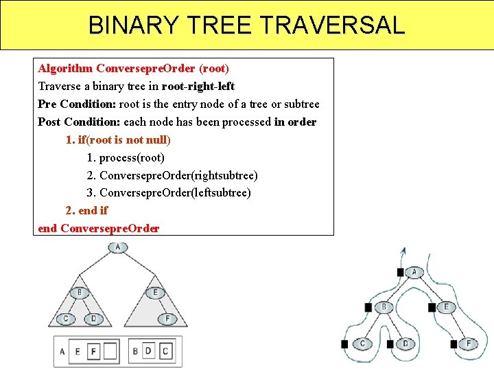
BINARY TREE TRAVERSAL Algorithm Conversepre. Order (root) Traverse a binary tree in root-right-left Pre Condition: root is the entry node of a tree or subtree Post Condition: each node has been processed in order 1. if(root is not null) 1. process(root) 2. Conversepre. Order(rightsubtree) 3. Conversepre. Order(leftsubtree) 2. end if end Conversepre. Order 47

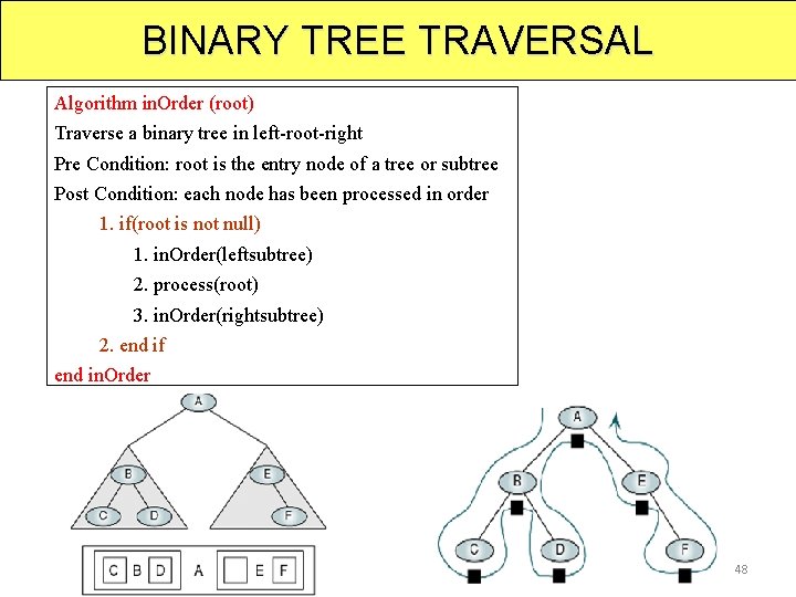
BINARY TREE TRAVERSAL Algorithm in. Order (root) Traverse a binary tree in left-root-right Pre Condition: root is the entry node of a tree or subtree Post Condition: each node has been processed in order 1. if(root is not null) 1. in. Order(leftsubtree) 2. process(root) 3. in. Order(rightsubtree) 2. end if end in. Order 48

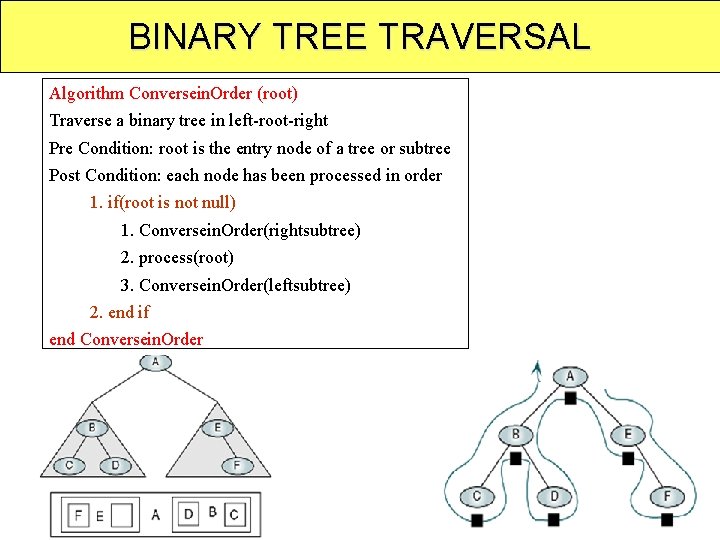
BINARY TREE TRAVERSAL Algorithm Conversein. Order (root) Traverse a binary tree in left-root-right Pre Condition: root is the entry node of a tree or subtree Post Condition: each node has been processed in order 1. if(root is not null) 1. Conversein. Order(rightsubtree) 2. process(root) 3. Conversein. Order(leftsubtree) 2. end if end Conversein. Order 49

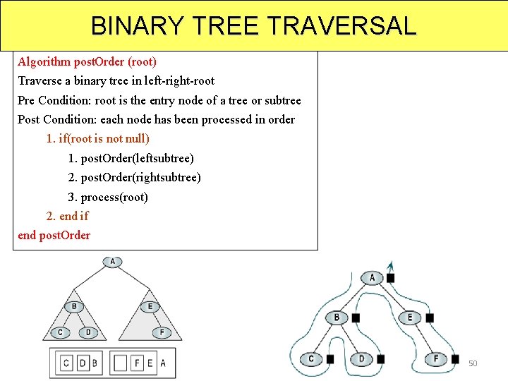
BINARY TREE TRAVERSAL Algorithm post. Order (root) Traverse a binary tree in left-right-root Pre Condition: root is the entry node of a tree or subtree Post Condition: each node has been processed in order 1. if(root is not null) 1. post. Order(leftsubtree) 2. post. Order(rightsubtree) 3. process(root) 2. end if end post. Order 50

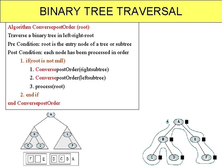
BINARY TREE TRAVERSAL Algorithm Conversepost. Order (root) Traverse a binary tree in left-right-root Pre Condition: root is the entry node of a tree or subtree Post Condition: each node has been processed in order 1. if(root is not null) 1. Conversepost. Order(rightsubtree) 2. Conversepost. Order(leftsubtree) 3. process(root) 2. end if end Conversepost. Order 51

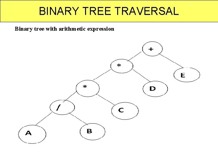
BINARY TREE TRAVERSAL Binary tree with arithmetic expression

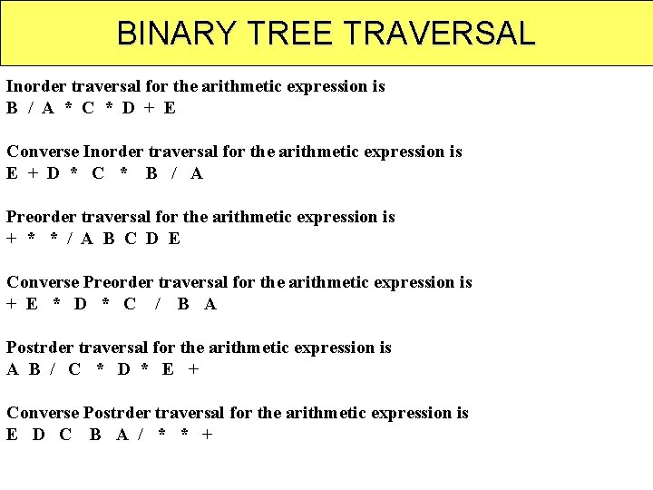
BINARY TREE TRAVERSAL Inorder traversal for the arithmetic expression is B / A * C * D + E Converse Inorder traversal for the arithmetic expression is E + D * C * B / A Preorder traversal for the arithmetic expression is + * * / A B C D E Converse Preorder traversal for the arithmetic expression is + E * D * C / B A Postrder traversal for the arithmetic expression is A B / C * D * E + Converse Postrder traversal for the arithmetic expression is E D C B A / * * +

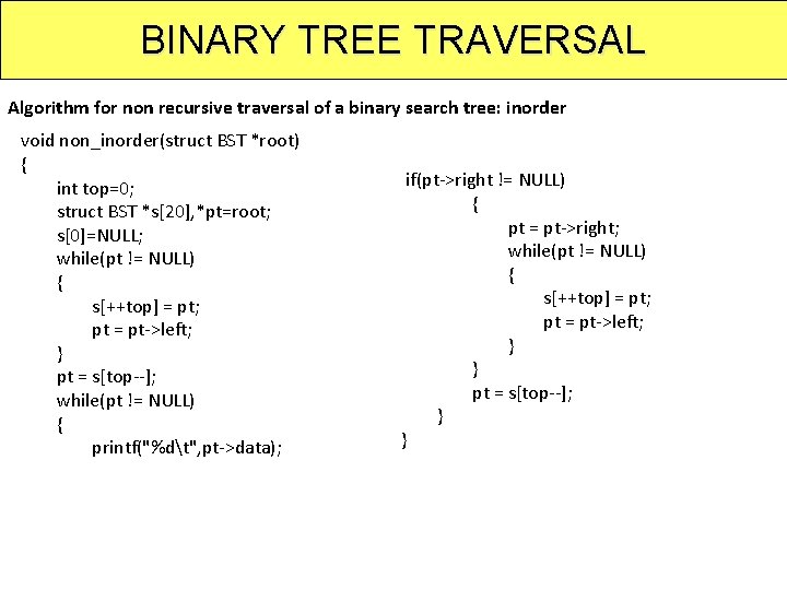
BINARY TREE TRAVERSAL Algorithm for non recursive traversal of a binary search tree: inorder void non_inorder(struct BST *root) { int top=0; struct BST *s[20], *pt=root; s[0]=NULL; while(pt != NULL) { s[++top] = pt; pt = pt->left; } pt = s[top--]; while(pt != NULL) { printf("%dt", pt->data); if(pt->right != NULL) { pt = pt->right; while(pt != NULL) { s[++top] = pt; pt = pt->left; } } pt = s[top--]; } }

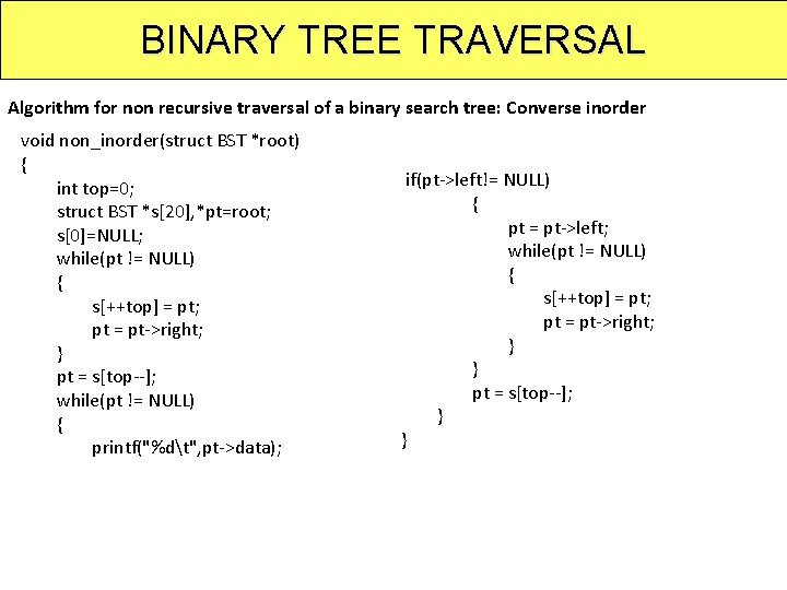
BINARY TREE TRAVERSAL Algorithm for non recursive traversal of a binary search tree: Converse inorder void non_inorder(struct BST *root) { int top=0; struct BST *s[20], *pt=root; s[0]=NULL; while(pt != NULL) { s[++top] = pt; pt = pt->right; } pt = s[top--]; while(pt != NULL) { printf("%dt", pt->data); if(pt->left!= NULL) { pt = pt->left; while(pt != NULL) { s[++top] = pt; pt = pt->right; } } pt = s[top--]; } }

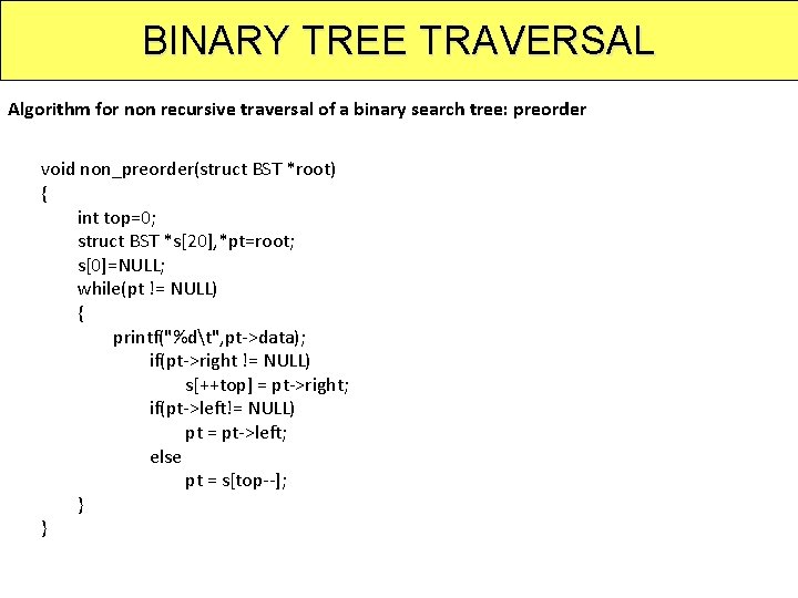
BINARY TREE TRAVERSAL Algorithm for non recursive traversal of a binary search tree: preorder void non_preorder(struct BST *root) { int top=0; struct BST *s[20], *pt=root; s[0]=NULL; while(pt != NULL) { printf("%dt", pt->data); if(pt->right != NULL) s[++top] = pt->right; if(pt->left!= NULL) pt = pt->left; else pt = s[top--]; } }

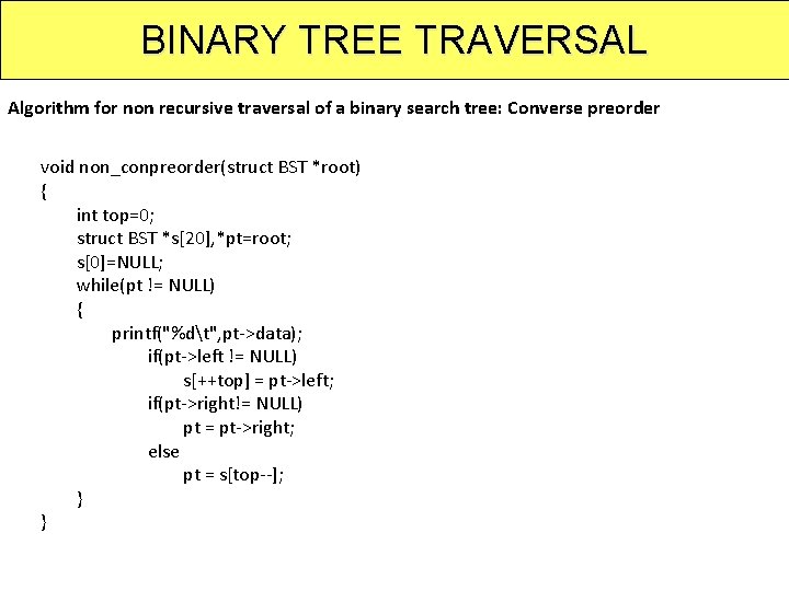
BINARY TREE TRAVERSAL Algorithm for non recursive traversal of a binary search tree: Converse preorder void non_conpreorder(struct BST *root) { int top=0; struct BST *s[20], *pt=root; s[0]=NULL; while(pt != NULL) { printf("%dt", pt->data); if(pt->left != NULL) s[++top] = pt->left; if(pt->right!= NULL) pt = pt->right; else pt = s[top--]; } }

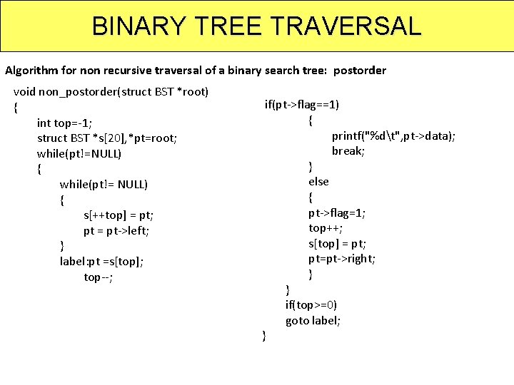
BINARY TREE TRAVERSAL Algorithm for non recursive traversal of a binary search tree: postorder void non_postorder(struct BST *root) { int top=-1; struct BST *s[20], *pt=root; while(pt!=NULL) { while(pt!= NULL) { s[++top] = pt; pt = pt->left; } label: pt =s[top]; top--; if(pt->flag==1) { printf("%dt", pt->data); break; } else { pt->flag=1; top++; s[top] = pt; pt=pt->right; } } if(top>=0) goto label; }

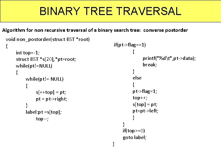
BINARY TREE TRAVERSAL Algorithm for non recursive traversal of a binary search tree: converse postorder void non_postorder(struct BST *root) { int top=-1; struct BST *s[20], *pt=root; while(pt!=NULL) { while(pt!= NULL) { s[++top] = pt; pt = pt->right; } label: pt =s[top]; top--; if(pt->flag==1) { printf("%dt", pt->data); break; } else { pt->flag=1; top++; s[top] = pt; pt=pt->left; } } if(top>=0) goto label; }

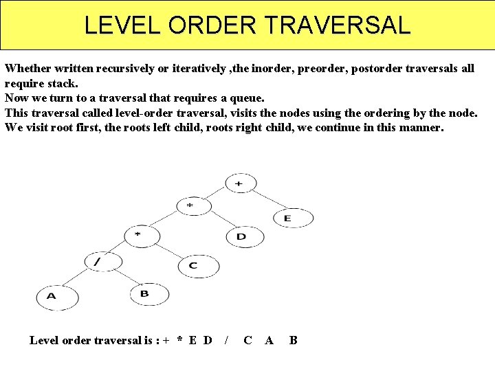
LEVEL ORDER TRAVERSAL Whether written recursively or iteratively , the inorder, preorder, postorder traversals all require stack. Now we turn to a traversal that requires a queue. This traversal called level-order traversal, visits the nodes using the ordering by the node. We visit root first, the roots left child, roots right child, we continue in this manner. Level order traversal is : + * E D / C A B

LEVEL ORDER TRAVERSAL Void levelorder(treepointer ptr) { int front=rear=0; treepointer queue[10]; if(!ptr) return; //empty tree addq(ptr); for(; ; ) { ptr=deleteq(); if(ptr) { printf(“%d”, ptr->data); if(ptr->leftchild) addq(ptr->leftchild) if(ptr->rightchild) addq(ptr->rightchild) } else break; } }

THREADED BINARY TREES Threads: 1. If we look carefully at the linked representation of any binary tree, we notice that there are more null links the actual pointers. 2. There are n+1 null links out of 2 n total links. 3. A. J. Perlis and C. Thornton have devised a cleverer way to make use of these null links. 4. They replace the null links by pointers called threads to other nodes in the tree. 5. To construct threads we use the following rules(assume ptr represents node) 1. If ptr->leftchild is null, replace ptr->leftchild with a pointer to the node that would be visited before ptr in an inorder traversal. (we replace the null link with a pointer to the inorder predessor of ptr). 2. If ptr->rightchild is null, replace ptr->rightchild with a pointer to the node that would be visited after ptr in an inorder traversal. . (we replace the null link with a pointer to the inorder successor of ptr).

PRIORITY QUEUES 1 of 8 1. A priority queue is a collection of zero or more elements. Each element has a priority or value. 2. Unlike the queues, the order of deleting from a priority queue is determined by the element priority. 3. Elements are removed/deleted either in increasing or decreasing order of priority rather than in the order in which they arrived in the queue. 63

PRIORITY QUEUES 2 of 8 Priority Queues are of two types: 1. Min priority queue or Ascending priority queue 2. Max priority queue or Descending priority queue 1. Min priority queue: Collection of elements in which the items can be inserted arbitrarily, but only smallest element can be removed. 1. Max priority queue: Collection of elements in which insertion of items can be in any order but only largest element can be removed. 64

PRIORITY QUEUES 4 of 8 ADT: A priority queue P supports the following methods: -size(): Return the number of elements in P -is. Empty(): Test whether P is empty or not -insert. Item(k, e): Insert a new element e with key k into P -min. Element(): Return an element of P with smallest key -min. Key(): Return the smallest key in P -remove. Min(): Remove from P and return an element with the smallest key. 65

PRIORITY QUEUES 4 of 8 ADT Max. Priority. Queue is Object: A collction of n>0 elements, each element has a key Function : for all q € Max. Priority. Queue , item € Element, n € integer Max. Priority. Queue Create(max_size) : : = create an empty priority queue. Boolean is. Empty(q, n) : : = if(n>0) return TRUE else return FALSE Element top(q, n) : : = if (!is. Empty(q, n) return an instance of the largest element in q else return error. Element pop(q, n) : : = if (!is. Empty(q, n) return an instance of the largest element in q and remove it from the heap else return error. Max. Priority. Queue push(q, item, n) : : = insert item into pq and return the resulting priority queue 66

PRIORITY QUEUES 3 of 8 APPLICATIONS: 1. The typical example of a priority queue is, scheduling the jobs in an operating system. Typically OS allocates priorities to jobs. The jobs are placed in the queue and position of the job in a priority queue determines their priority. 2. In network communication, the priority queue is used to manage the limited bandwidth for transmission. 3. In simulation modeling, the priority queue is used to manage the discrete events. Selling the services of machine 4. 67

PRIORITY QUEUES 4 of 8 If Priority Queue is unorder linear list: is. Empty () : takes O(1) time top() : takes Ø(n) time push() : O(1) pop() : Ø(n) In Max Heap: is. Empty () & top() : takes O(1) time push() : pop() : O(log n) 68

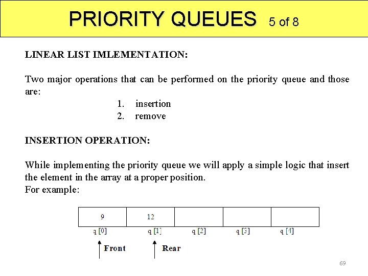
PRIORITY QUEUES 5 of 8 LINEAR LIST IMLEMENTATION: Two major operations that can be performed on the priority queue and those are: 1. insertion 2. remove INSERTION OPERATION: While implementing the priority queue we will apply a simple logic that insert the element in the array at a proper position. For example: 69

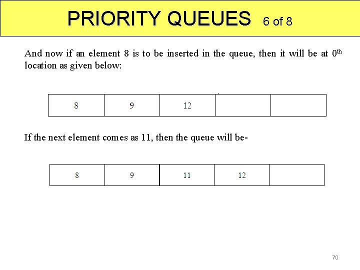
PRIORITY QUEUES 6 of 8 And now if an element 8 is to be inserted in the queue, then it will be at 0 th location as given below: If the next element comes as 11, then the queue will be- 70

PRIORITY QUEUES Pseudo code: void insert. New. Item(int q[], int rear, int front) 1. { 2. read item; 3. if(rear = max-1) cout<<”Queue overflow”; 4. else 5. if(front == -1) 6. front ++; 7. j=rear; 8. while(j>0 && item<q[j]) 9. { 10. q[j+1] = q[j]; 11. j--; 12. } 13. q[j+1] = item; 14. rear = rear+1; 15. return rear; 16. } 7 of 8 71

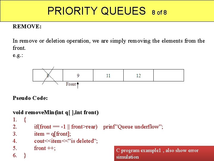
PRIORITY QUEUES 8 of 8 REMOVE: In remove or deletion operation, we are simply removing the elements from the front. e. g. : Pseudo Code: void remove. Min(int q[ ], int front) 1. { 2. if(front == -1 || front>rear) prinf”Queue underflow”; 3. item = q[front]; 4. cout<<item<<”is deleted”; 5. front ++; C program example 1 , also show error 72 6. } simulation

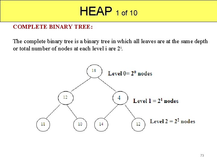
HEAP 1 of 10 COMPLETE BINARY TREE: The complete binary tree is a binary tree in which all leaves are at the same depth or total number of nodes at each level i are 2 i. 73

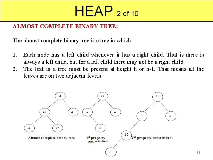
HEAP 2 of 10 ALMOST COMPLETE BINARY TREE: The almost complete binary tree is a tree in which – 1. Each node has a left child whenever it has a right child. That is there is always a left child, but for a left child there may not be a right child. 2. The leaf in a tree must be present at height h or h-1. That means all the leaves are on two adjacent levels. 74

HEAP 3 of 10 DEFINITION: Heap is a complete binary tree or an almost complete binary tree in which every parent node be either greater or less than its child nodes. Heap is a tree data structure denoted by either a max heap or a min heap. 1. A max (min) tree is a tree in which the key value in each node is no smaller ( larger) than the key values in its children (if any). 2. A max heap is a complete binary tree that is also a max tree. 3. A min heap is a complete binary tree that is also a min tree. 75

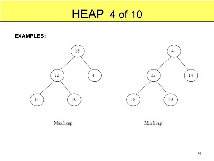
HEAP 4 of 10 EXAMPLES: 76

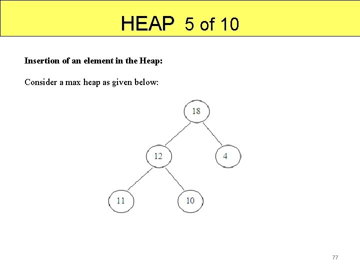
HEAP 5 of 10 Insertion of an element in the Heap: Consider a max heap as given below: 77

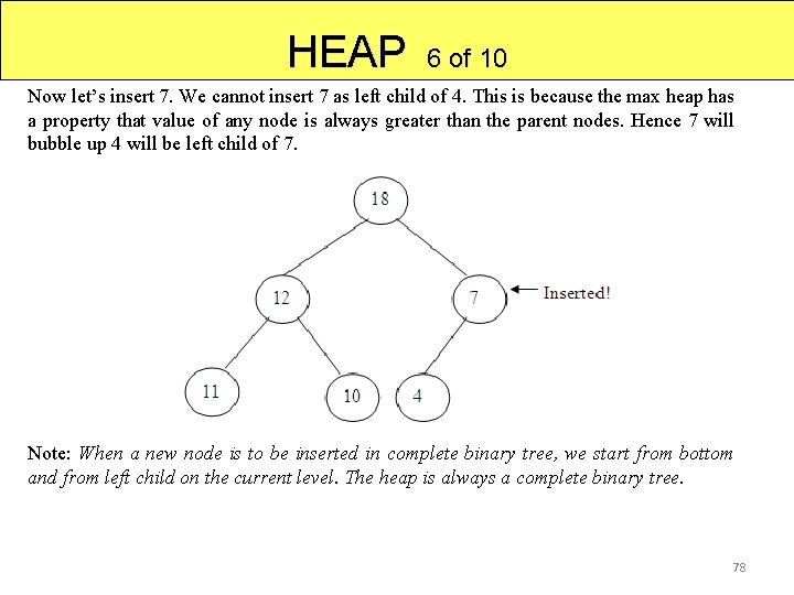
HEAP 6 of 10 Now let’s insert 7. We cannot insert 7 as left child of 4. This is because the max heap has a property that value of any node is always greater than the parent nodes. Hence 7 will bubble up 4 will be left child of 7. Note: When a new node is to be inserted in complete binary tree, we start from bottom and from left child on the current level. The heap is always a complete binary tree. 78

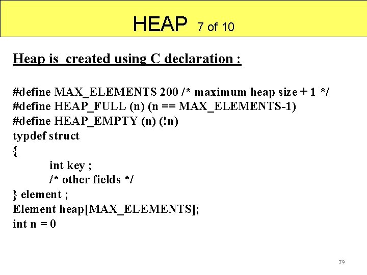
HEAP 7 of 10 Heap is created using C declaration : #define MAX_ELEMENTS 200 /* maximum heap size + 1 */ #define HEAP_FULL (n) (n == MAX_ELEMENTS-1) #define HEAP_EMPTY (n) (!n) typdef struct { int key ; /* other fields */ } element ; Element heap[MAX_ELEMENTS]; int n = 0 79

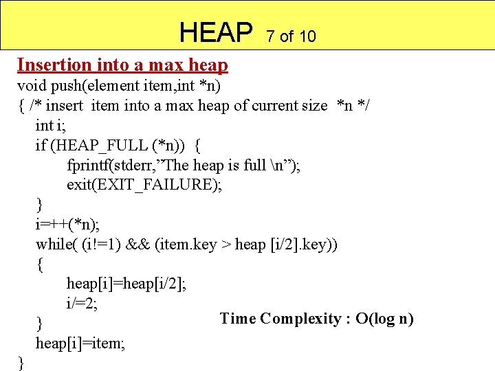
HEAP 7 of 10 Insertion into a max heap void push(element item, int *n) { /* insert item into a max heap of current size *n */ int i; if (HEAP_FULL (*n)) { fprintf(stderr, ”The heap is full n”); exit(EXIT_FAILURE); } i=++(*n); while( (i!=1) && (item. key > heap [i/2]. key)) { heap[i]=heap[i/2]; i/=2; Time Complexity : O(log n) } heap[i]=item; }

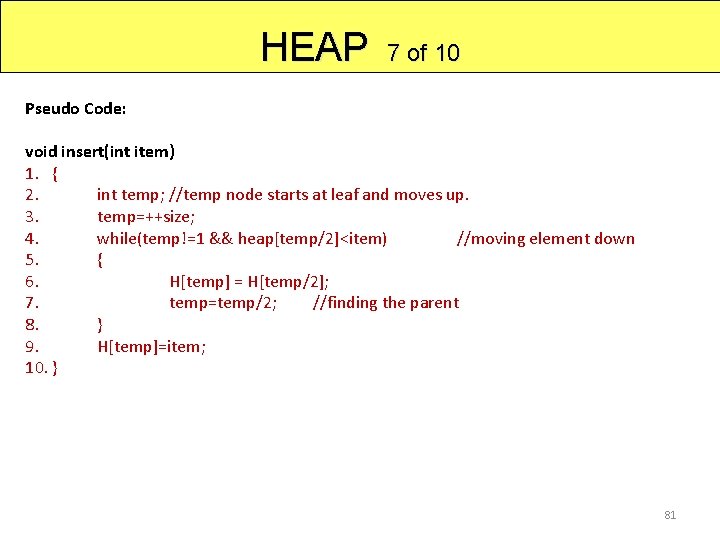
HEAP 7 of 10 Pseudo Code: void insert(int item) 1. { 2. int temp; //temp node starts at leaf and moves up. 3. temp=++size; 4. while(temp!=1 && heap[temp/2]<item) //moving element down 5. { 6. H[temp] = H[temp/2]; 7. temp=temp/2; //finding the parent 8. } 9. H[temp]=item; 10. } 81

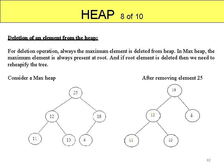
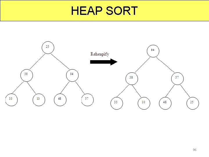
HEAP 8 of 10 Deletion of an element from the heap: For deletion operation, always the maximum element is deleted from heap. In Max heap, the maximum element is always present at root. And if root element is deleted then we need to reheapify the tree. Consider a Max heap After removing element 25 82

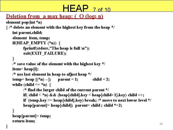
HEAP 7 of 10 Deletion from a max heap: ( O (log 2 n) element pop(int *n) { /* delete an element with the highest key from the heap */ int parent, child; element item, temp; if(HEAP_EMPTY (*n)) { fprintf(stderr, ”The heap is full n”); exit(EXIT_FAILURE); } /* save value of the element with the highest key */ item= heap[i]; /* use last element in heap to afjust heap */ temp= heap [(*n) --]; parent = 1; child = 2; while (child <= *n) { /* find the larger child of the current parent */ if( child < *n) && (heap[child]. key < heap[child+1]. key) child ++; if (temp. key >= heap[child]. key) break; /* move to next lower level */ heap[parent]= heap[child]; parent= child ; child *=2; } heap[parent]= temp; return item; } 83

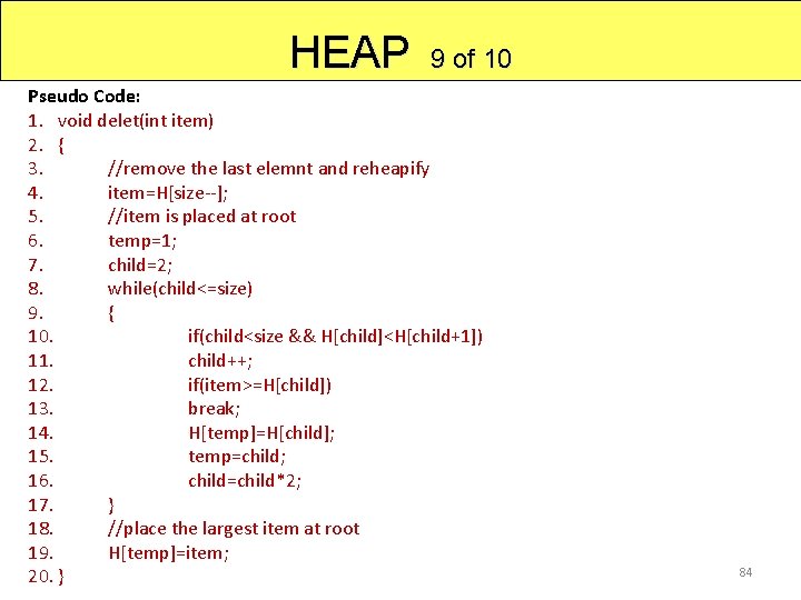
HEAP 9 of 10 Pseudo Code: 1. void delet(int item) 2. { 3. //remove the last elemnt and reheapify 4. item=H[size--]; 5. //item is placed at root 6. temp=1; 7. child=2; 8. while(child<=size) 9. { 10. if(child<size && H[child]<H[child+1]) 11. child++; 12. if(item>=H[child]) 13. break; 14. H[temp]=H[child]; 15. temp=child; 16. child=child*2; 17. } 18. //place the largest item at root 19. H[temp]=item; 20. } 84

HEAP 10 of 10 APPLICATIONS 1. Heap is used in sorting algorithms. One such algorithm using heap is known as heap sort. 2. In priority queue implementation the heap is used. 85

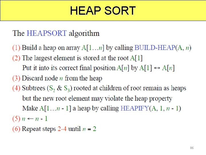
HEAP SORT 86

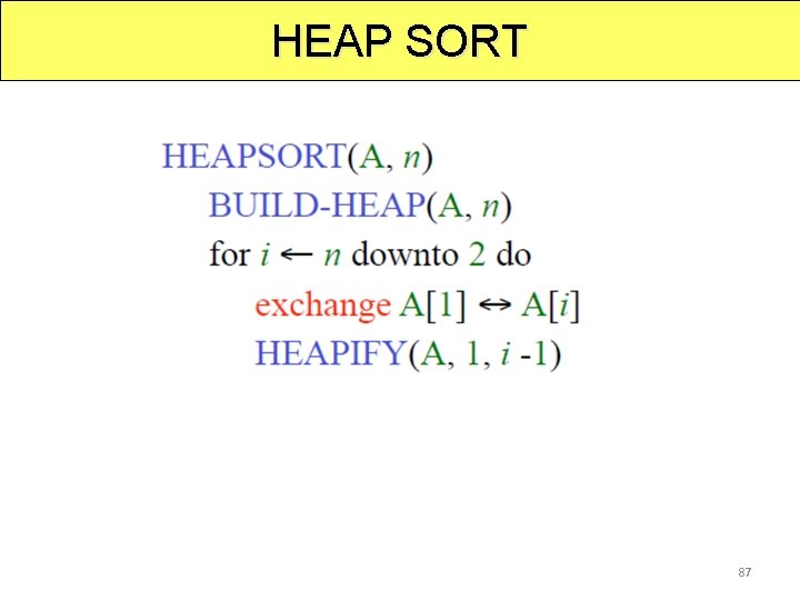
HEAP SORT 87

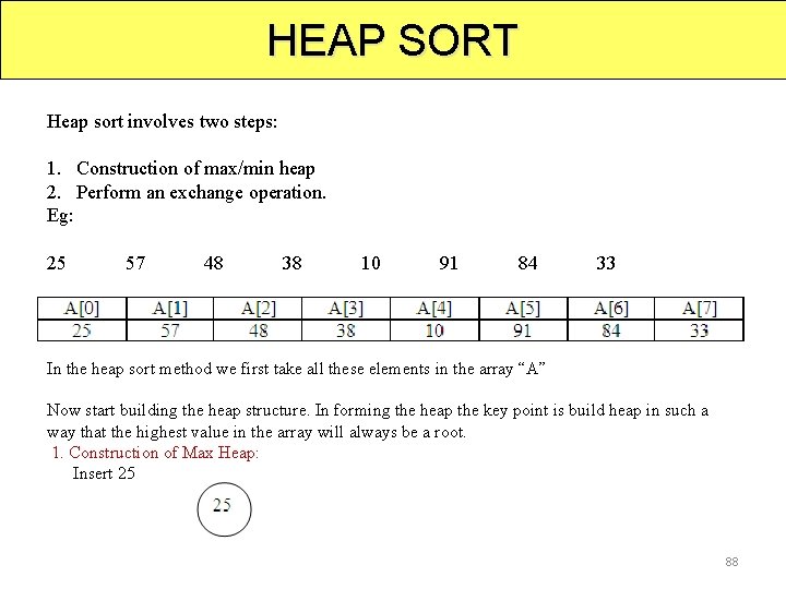
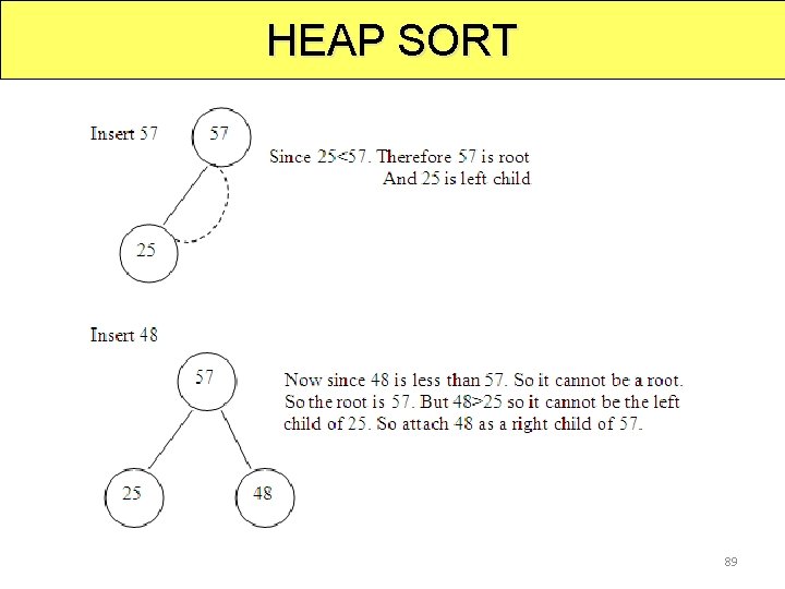
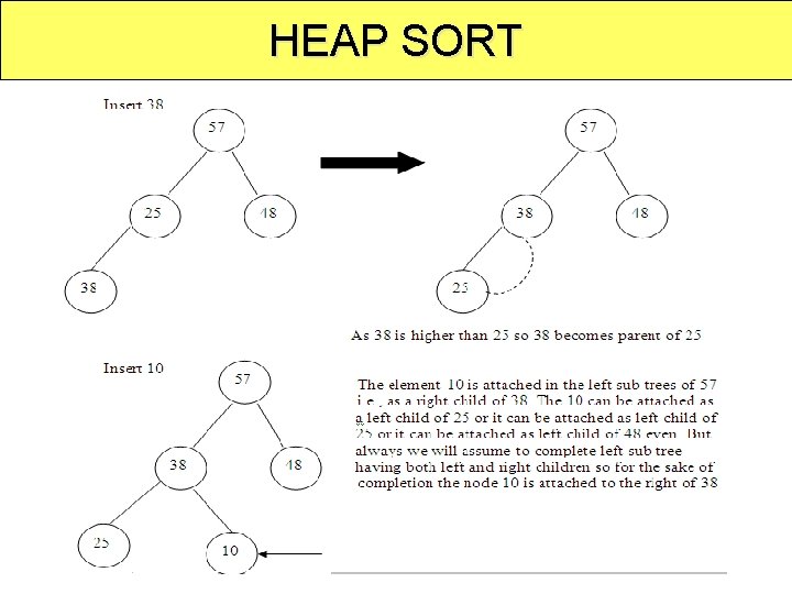
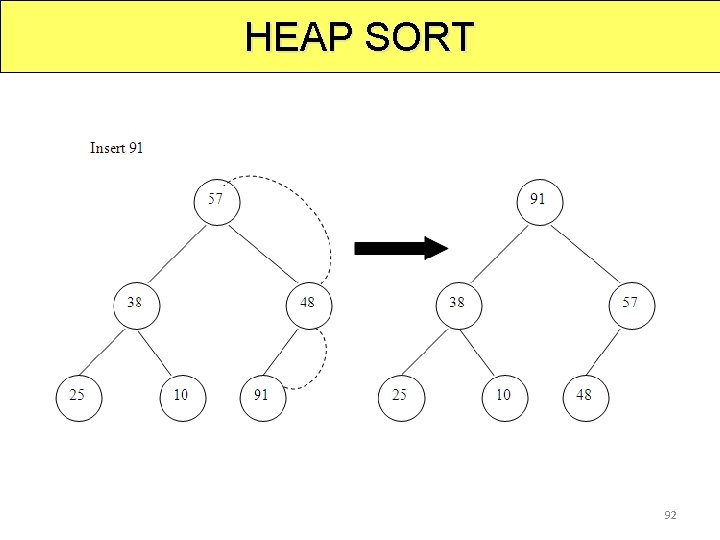
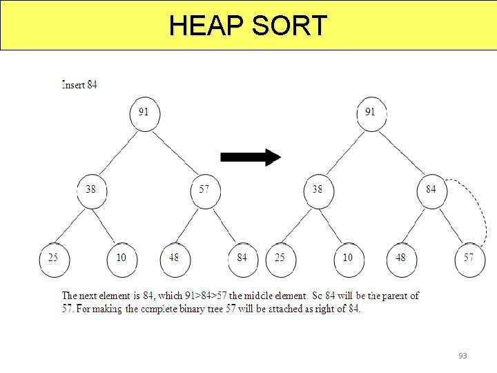
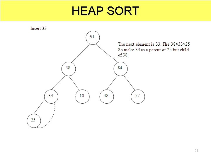
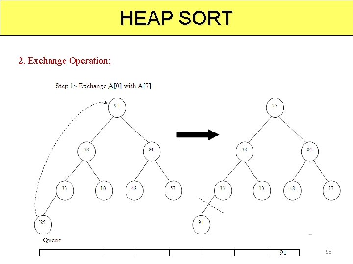
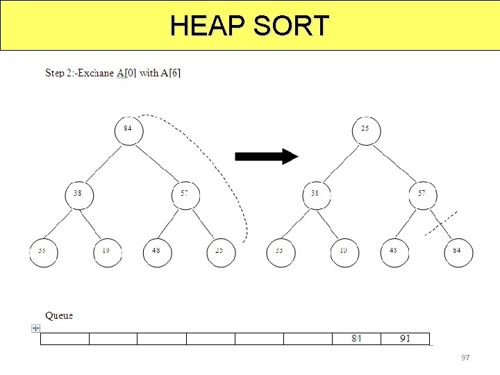
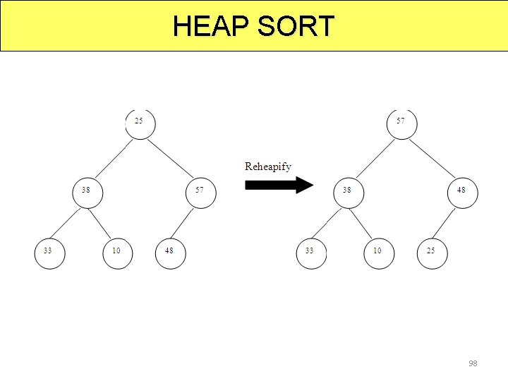
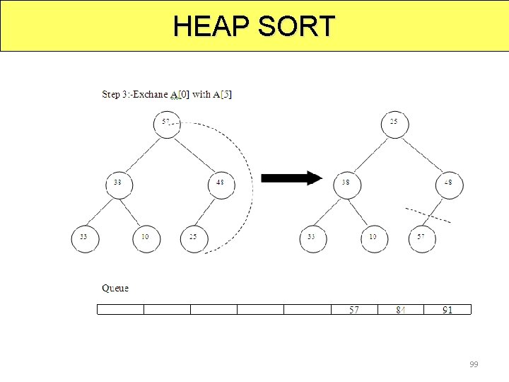
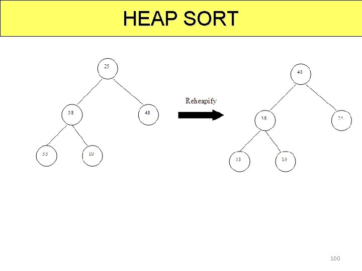
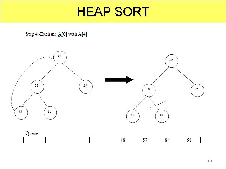
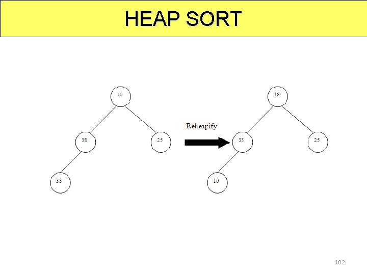
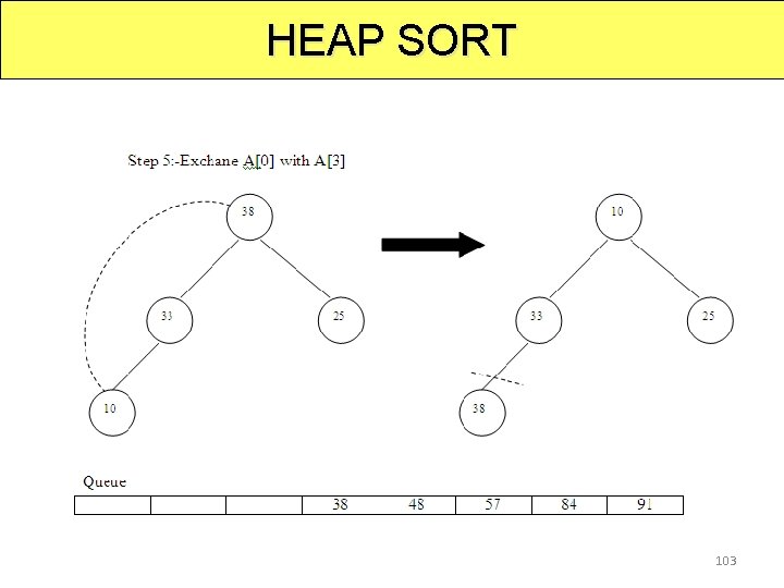
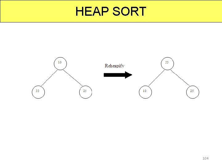
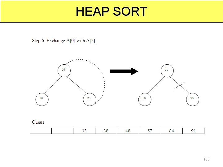
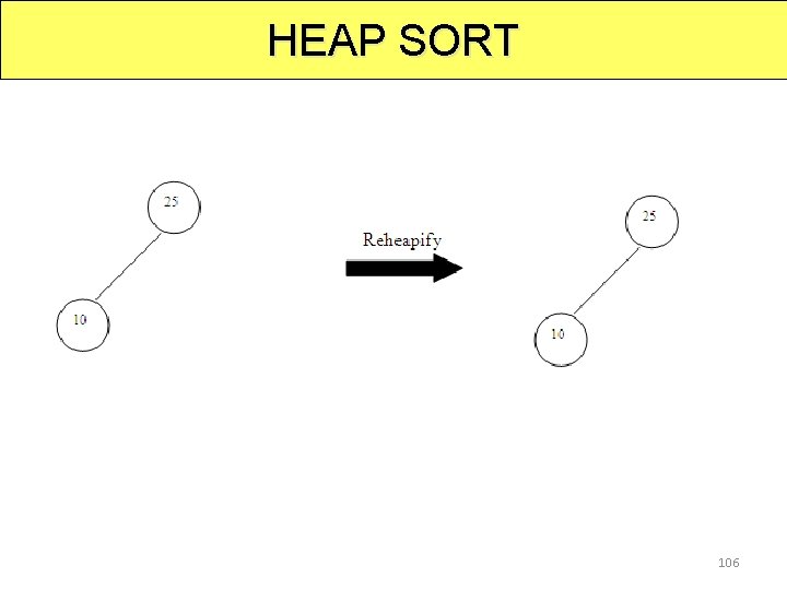
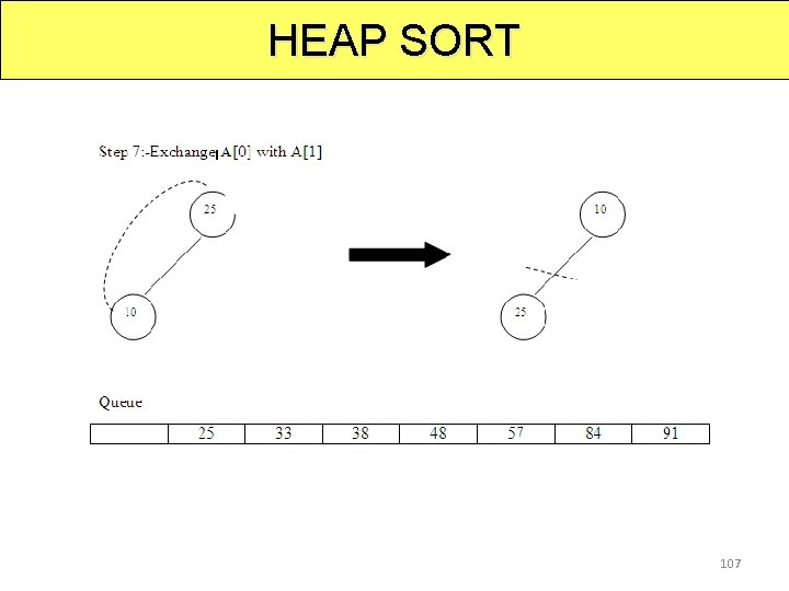
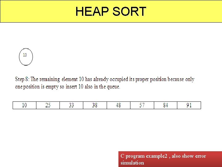
HEAP SORT Heap sort involves two steps: 1. Construction of max/min heap 2. Perform an exchange operation. Eg: 25 57 48 38 10 91 84 33 In the heap sort method we first take all these elements in the array “A” Now start building the heap structure. In forming the heap the key point is build heap in such a way that the highest value in the array will always be a root. 1. Construction of Max Heap: Insert 25 88

HEAP SORT 89

HEAP SORT 90

HEAP SORT 91

HEAP SORT 92

HEAP SORT 93

HEAP SORT 94

HEAP SORT 2. Exchange Operation: 95

HEAP SORT 96

HEAP SORT 97

HEAP SORT 98

HEAP SORT 99

HEAP SORT 100

HEAP SORT 101

HEAP SORT 102

HEAP SORT 103

HEAP SORT 104

HEAP SORT 105

HEAP SORT 106

HEAP SORT 107

HEAP SORT C program example 2 , also show error 108 simulation

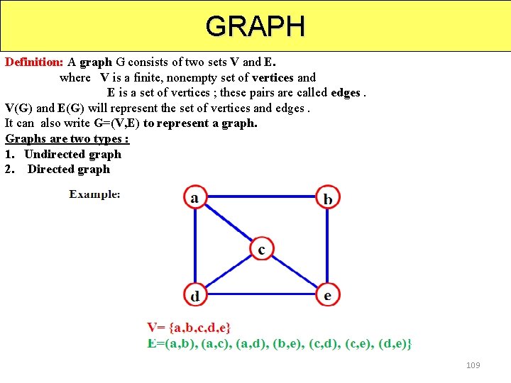
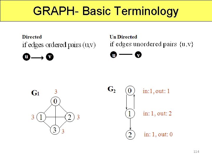
GRAPH Definition: A graph G consists of two sets V and E. where V is a finite, nonempty set of vertices and E is a set of vertices ; these pairs are called edges. V(G) and E(G) will represent the set of vertices and edges. It can also write G=(V, E) to represent a graph. Graphs are two types : 1. Undirected graph 2. Directed graph 109

GRAPH- Basic Terminology The restrictions on Graph: 1. It mat not have edge from vertex, v , back to itself. That is, edges of the form (V, V) and <V, V> are not legal. such edges are known as self edges or self loops. Its data object referred to as a graph with loops 2. It may not have multiple occurrences of the same edge. if it remove then the graph is a multigraph The no of distinct unordered pairs (u, v)with u not equal to v in a graph of n vertices is n(n 1)/2. This is the maximum no of edges. An unordered graph , with n vertices with exactly n(n-1)/2 edges is said to be Complete A directed graph on n vertices , the maximum no edges is n(n-1) 110

GRAPH- Basic Terminology ØA directed graph or digraph is one in which the edges have a direction. Ø An undirected graph is one in which the edges do not have a direction. Ø The size of a graph is the number of nodes in it Ø The empty graph has size zero (no nodes). ØIf two nodes are connected by an edge, they are neighbors (and the nodes are adjacent to each other). ØA path is a sequence of nodes such that each node (but the last) is the predecessor of the next node in the list. Example: If v 1, v 2, . . . , vk are vertices then vi and vi+1 should be consecutive. A length of the path is the number of edges on it. A simple path is a path in which all vertices except possibly the first & last are distinct. 111

GRAPH- Basic Terminology ØA directed graph or digraph is one in which the edges have a direction. Ø An undirected graph is one in which the edges do not have a direction. Ø The size of a graph is the number of nodes in it Ø The empty graph has size zero (no nodes). ØIf two nodes are connected by an edge, they are neighbors (and the nodes are adjacent to each other). ØA path is a sequence of nodes such that each node (but the last) is the predecessor of the next node in the list. Example: If v 1, v 2, . . . , vk are vertices then vi and vi+1 should be consecutive. ØThe degree of a node is the number of edges it has. ØFor directed graphs: ØThe in-degree of a node is the number of in-edges it has. ØThe out-degree of a node is the number of out-edges it has. 112

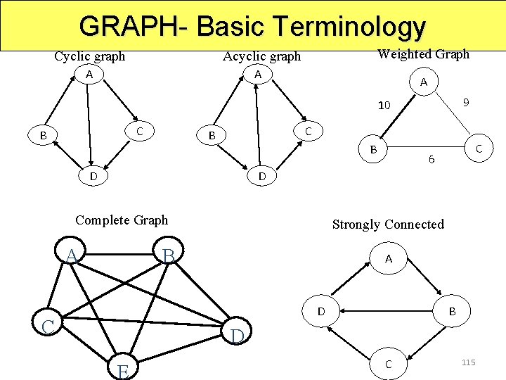
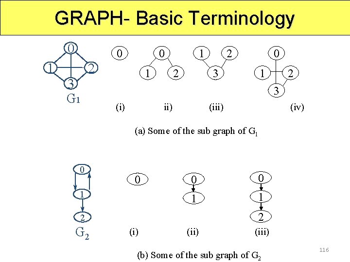
GRAPH- Basic Terminology ØAn undirected graph is connected if there is a path from every node to every other node. ØA directed graph is strongly connected if there is a path from every node to every other node. ØA simple path is a path in which all the vertices, except possibly the first and last vertices, are distinct. ØA cycle in G is a simple path in which the first and last vertices are the same. ØA graph without cycles is called acyclic graph. ØSub graph is a graph with subset of vertices and edges of a graph. ØA graph is called a simple graph if it has no loops and no parallel edges. ØA graph is termed as weighted graph if all the edges in it are labeled with some weights. ØA complete graph is a graph if there is a path from every node to every other node. 113

GRAPH- Basic Terminology 114

GRAPH- Basic Terminology Cyclic graph Weighted Graph Acyclic graph A A A 9 10 C B B C 6 D D Complete Graph A Strongly Connected B A D C B D E C 115

GRAPH- Basic Terminology 0 0 1 0 2 3 G 1 1 1 2 2 3 0 1 2 3 (i) ii) (iii) (iv) (a) Some of the sub graph of G 1 0 1 2 G 2 0 0 0 1 1 2 (i) (iii) (b) Some of the sub graph of G 2 116

ADT Graph is Object: a nonempty set of vertices and a set of undirected egdes , where each edge is a pair of vertices. Functions : for all graph € Graph , v , v 1 and v 2 € Vertices. Graph Create () : : = return an empty graph Graph Insert. Vertex(graph, v) : : =return graph with v vertex inserted v has no incident edges. Graph Insert. Edge(graph, v 1, v 2) : : =return graph with new edges between v 1 &v 2. Graph Delete. Vertex(graph, v) : : =return graph in which v inserted and al the edges incident to it are removed. Graph Delete. Edge(graph, v 1, v 2) : : =return graph in which edge ( v 1, v 2. ) is removed. Leave the incident nodes in the graph Boolean Is. Empty(graph) : : = List Adjacent(graph, v) 117

REPRESENTATION There are two ways of representing a graph in memory: ØSequential Representation by means of Adjacency Matrix. ØLinked Representation by means of Linked List. 118

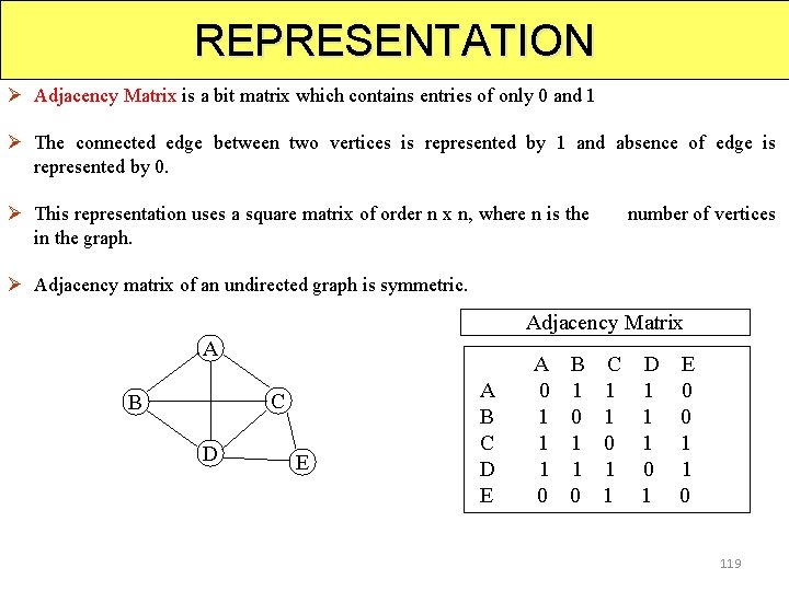
REPRESENTATION Ø Adjacency Matrix is a bit matrix which contains entries of only 0 and 1 Ø The connected edge between two vertices is represented by 1 and absence of edge is represented by 0. Ø This representation uses a square matrix of order n x n, where n is the number of vertices in the graph. Ø Adjacency matrix of an undirected graph is symmetric. Adjacency Matrix A C B D E A B C D E A 0 1 1 1 0 B 1 0 1 1 0 C 1 1 0 1 1 D 1 1 1 0 1 E 0 0 1 1 0 119

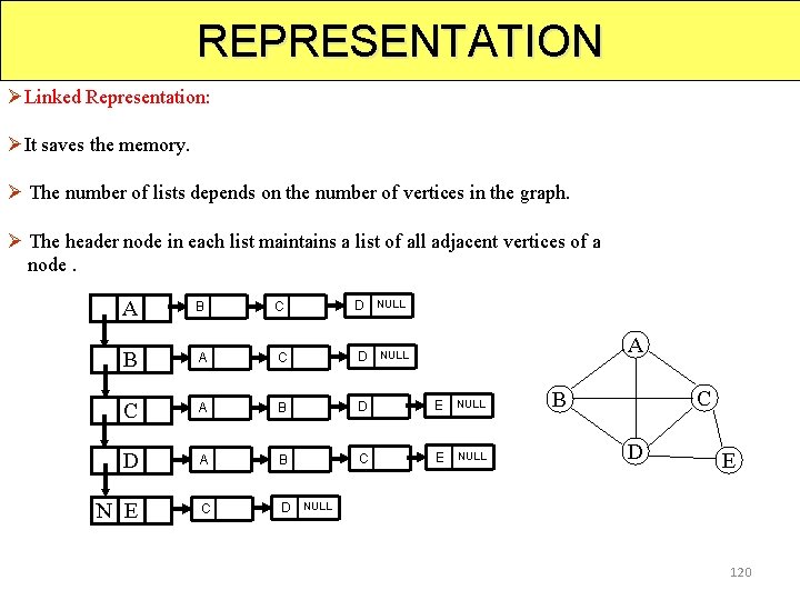
REPRESENTATION ØLinked Representation: ØIt saves the memory. Ø The number of lists depends on the number of vertices in the graph. Ø The header node in each list maintains a list of all adjacent vertices of a node. A B C D NULL B A C D NULL C A B D E NULL D A B C E NULL N E C D NULL A C B D E 120

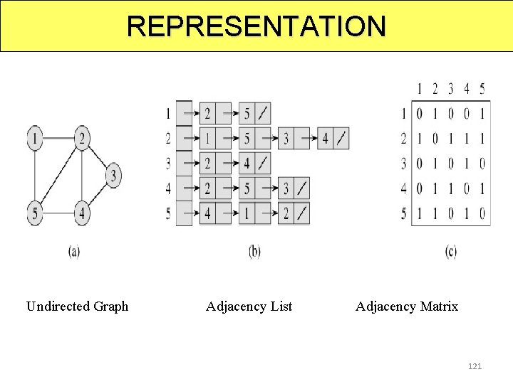
REPRESENTATION Undirected Graph Adjacency List Adjacency Matrix 121

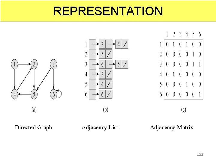
REPRESENTATION Directed Graph Adjacency List Adjacency Matrix 122

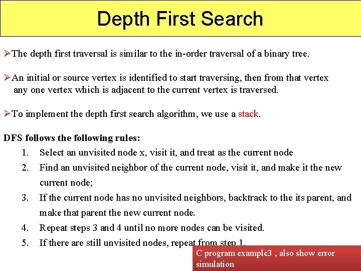
Depth First Search ØThe depth first traversal is similar to the in-order traversal of a binary tree. ØAn initial or source vertex is identified to start traversing, then from that vertex any one vertex which is adjacent to the current vertex is traversed. ØTo implement the depth first search algorithm, we use a stack. DFS follows the following rules: 1. Select an unvisited node x, visit it, and treat as the current node 2. Find an unvisited neighbor of the current node, visit it, and make it the new current node; 3. If the current node has no unvisited neighbors, backtrack to the its parent, and make that parent the new current node. 4. Repeat steps 3 and 4 until no more nodes can be visited. 5. If there are still unvisited nodes, repeat from step 1. C program example 3 , also show error 123 simulation

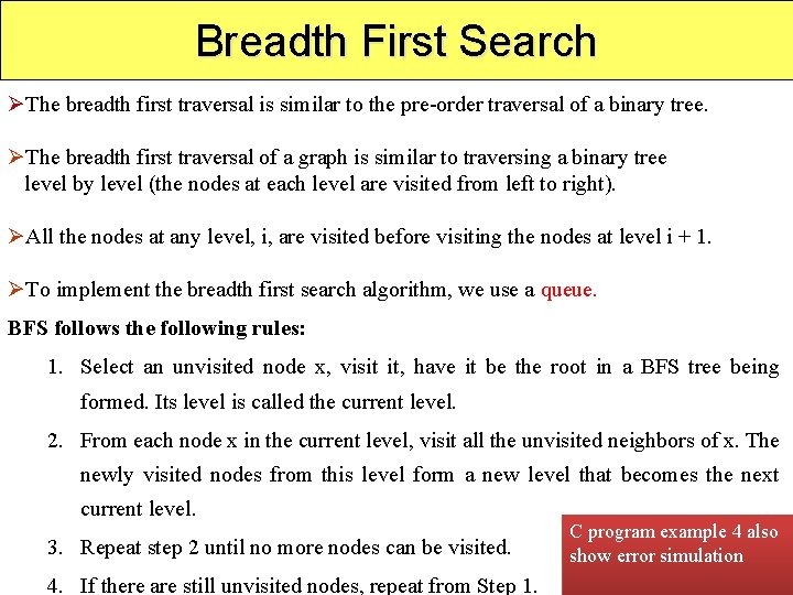
Breadth First Search ØThe breadth first traversal is similar to the pre-order traversal of a binary tree. ØThe breadth first traversal of a graph is similar to traversing a binary tree level by level (the nodes at each level are visited from left to right). ØAll the nodes at any level, i, are visited before visiting the nodes at level i + 1. ØTo implement the breadth first search algorithm, we use a queue. BFS follows the following rules: 1. Select an unvisited node x, visit it, have it be the root in a BFS tree being formed. Its level is called the current level. 2. From each node x in the current level, visit all the unvisited neighbors of x. The newly visited nodes from this level form a new level that becomes the next current level. 3. Repeat step 2 until no more nodes can be visited. 4. If there are still unvisited nodes, repeat from Step 1. C program example 4 also show error simulation 124

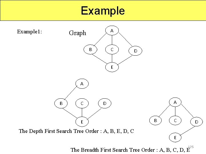
Example 1: A Graph B C D E A B C A D E B C D The Depth First Search Tree Order : A, B, E, D, C E 125 The Breadth First Search Tree Order : A, B, C, D, E

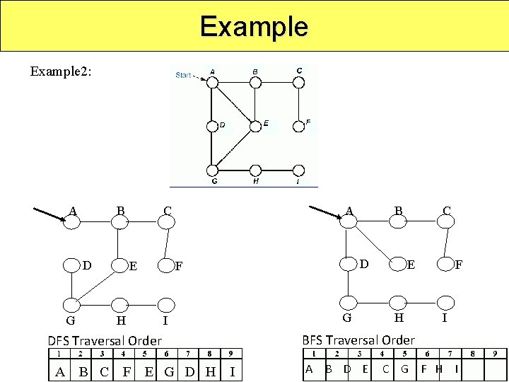
Example 2: A B D G A C E H D F I DFS Traversal Order A B C F E G D H I B G C E H F I BFS Traversal Order A B D E C G F H I