UNIT1 Objectives Algorithm Specification Recursive algorithms Data Abstraction

UNIT-1 Objectives • Algorithm Specification • Recursive algorithms • Data Abstraction • Performance analysis • Asymptotic Notation • Introduction to Linear and Non Linear data structures • Singly Linked list • Circularly linked lists • Double Linked list • Representation of single, two dimensional arrays • Sparse matrices-array and linked representations 1

ALGORITHM Definition: An Algorithm is a method of representing the step-by-step procedure for solving a problem. It is a method of finding the right answer to a problem or to a different problem by breaking the problem into simple cases. It must possess the following properties: Finiteness: An algorithm should terminate in a finite number of steps. Definiteness: Each step of the algorithm must be precisely (clearly) stated. Effectiveness: Each step must be effective. i. e; it should be easily convertible into program statement and can be performed exactly in a finite amount of time. Generality: Algorithm should be complete in itself, so that it can be used to solve all problems of given type for any input data. Input/Output: Each algorithm must take zero, one or more quantities as input data and gives one of more output values. 2

Recursive Algorithms 1 of 10 Definition: • A recursive algorithm is one in which objects are defined in terms of other objects of the same type. Advantages: • Simplicity of code • Easy to understand Disadvantages: • Memory • Speed 3

Recursive Algorithms 2 of 10 All recursive algorithms must obey three important laws: 1. A recursive algorithm must have a base case. 2. A recursive algorithm must change its state and move toward the base case. 3. A recursive algorithm must call itself, recursively Types of Recursions: 1. Direct Recursion 2. Indirect Recursion 3. Tail Recursion 4. Linear Recursion 5. Tree Recursion 4

Recursive Algorithms 3 of 10 1. Direct Recursion A C function is directly recursive if it contains an explicit call to itself Int foo (int x) { if ( x <= 0 ) return x; return foo ( x – 1); } 5

Recursive Algorithms 4 of 10 2. Indirect Recursion A C function foo 1 is indirectly recursive if it contains a call to another function that ultimately calls foo 1. int foo 1(int x){ if (x <= 0) return x; return foo 2 (x); } int foo 2 (int y) { return foo 1(y – 1); } 6

Recursive Algorithms 5 of 10 3. Tail Recursion A recursive function is said to be tail recursive if there is no pending operations performed on return from a recursive call Tail recursive functions are often said to “return the value of the last recursive call as the value of the function” Tail recursive factorial is non-tail recursive int fact_Trec (int n, int result) { if (n == 1) return result; return fact_Trec (n – 1, n * result); } int factorial (int n) { if (n == 0) return 1; return n * factorial(n – 1); } factorial (int n) { return fact_Trec (n, 1); } Note: The “pending operation” (namely the multiplication) to be performed on return from each recursive call 7

Recursive Algorithms 6 of 10 4. Linear Recursion A recursive function is said to be linearly recursive when no pending operation invokes another recursive call to the function. int factorial (int n) { if (n == 0) return 1; return n * factorial ( n – 1); } 8

Recursive Algorithms 7 of 10 5. Tree Recursion A recursive function is said to be tree recursive (or nonlinearly recursive when the pending operation does invoke another recursive call to the function. The Fibonacci function fib provides a classic example of tree recursion. // Note how the pending operation (the +) // needs a 2 nd recursive call to fib int fib(int n) { if (n == 0) return 0; if (n == 1) return 1; return ( fib ( n – 1 ) + fib ( n – 2 ) ); } 9

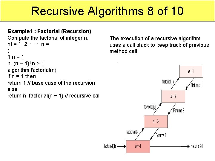
Recursive Algorithms 8 of 10 Example 1 : Factorial (Recursion) Compute the factorial of integer n: n! = 1 2 · · · n = ( 1 n = 1 n (n − 1)! n > 1 algorithm factorial(n) if n = 1 then return 1 // base case of the recursion else return n factorial(n − 1) // recursive call The execution of a recursive algorithm uses a call stack to keep track of previous method call 10

Recursive Algorithms 9 of 10 Example 2: Factorial (Tail-Recursion) The previous factorial algorithm is augmented recursive, i. e. it can be replaced by a tail-recursion 11

Recursive Algorithms 10 of 10 Example 3: Factorial (Iteration) The tail-recursive factorial algorithm can be replaced by a simple iterative loop 12

Data Abstraction The basic data types includes char , int , float & double. Some data types may be modified by keywords short , long , unsigned Two mechanisms for grouping data together: 1. Arrays 2. Structures Data types: It is a collection of objects & set of operations that act on those objects. int consists of objects { 0 , +1 , -1 , +2 , -2 , INT_MAX, INT_MIN } INT_MAX : largest integer on machine INT_MIN: smallest integer on machine It includes in <limits. h> 13

Data Abstraction Abstract Data Type(ADT): It is a data type i. e, organised in such a way that the specification of the objects & the specification of the operations on the objects is separated from the representation of the objects & implementation of the operations. e. g : Ada have packages C++ have class The functions of a data types into several categories: 1. Creator / constructor 2. Transformers 3. Observers / reporters 14

Data Abstraction 1. Creator / constructor: These functions create a new instance of the designed type. 2. Transformers : These functions also create an instance of the designed type generally by using 1 / more other instances. 3. Observers / reporters: These functions provide information about an instance of the type , but they do not change the instance 15

PERFORMANCE ANALYSIS 1 of 4 When several algorithms can be designed for the solution of a problem, there arises the need to determine which among them is the best. The efficiency of a program or an algorithm is measured by computing – • Time Complexity • Space Complexity 16

PERFORMANCE ANALYSIS 2 of 4 Time Complexity • The time complexity of an algorithm is a function of the running time of the algorithm. • The time complexity is therefore given in terms of frequency count. • Frequency count is basically a count denoting number of times of execution of statement. Example 1: 1 2 3 4 5 6 7 Algorithm Message(n) { for i=1 to n do { write(“Hello”); } } 0 0 n+1 0 n 0 0 total frequency count 2 n+1 While computing the time complexity we will neglect all the constants, hence ignoring 2 and 1 we will get n. Hence the time complexity becomes O(n). 17

PERFORMANCE ANALYSIS 3 of 4 Space Complexity • The space complexity can be defined as amount of memory required by an algorithm to run. • To compute the space complexity we use two factors: constant and instance characteristics. The space requirement S(p) can be given as S(p) = C + Sp where C is a constant i. e. , fixed part and it denotes the space of inputs and outputs. This space is an amount of space taken by instruction, variables and identifiers. Sp is a space dependent upon instance characteristics. This is a variable part whose space requirement depend on particular problem instance. 18

PERFORMANCE ANALYSIS 4 of 4 Example: 1 Algorithm add(a, b, c) { return a+b+c; } If we assume a, b, c occupy one word size then total size comes to be 3 S(p) = C (since C=3) Example: 2 Algorithm add(x, n) { sum=0. 0; for i= 1 to n do sum: =sum+x[i]; return sum; } The n space required for x[], one space for n, one for i, and one for sum S(p) ≥ (n+3) 19

Asymptotic Notations: 1 of 5 • To choose the best algorithm, we need to check efficiency of each algorithm. The efficiency can be measured by computing time complexity of each algorithm. Asymptotic notation is a shorthand way to represent the time complexity. • Using asymptotic notations we can give time complexity as “fastest possible”, “slowest possible” or “average time”. • Various notations such as Ω, θ, O used are called asymptotic notations. 20

Asymptotic Notations: 2 of 5 Big Oh Notation Big Oh notation denoted by ‘O’ is a method of representing the upper bound of algorithm’s running time. Using big oh notation we can give longest amount of time taken by the algorithm to complete. Definition: Let, f(n) and g(n) are two non-negative functions. And if there exists an integer n 0 and constant C such that C > 0 and for all integers n > n 0, f(n) ≤ c*g(n), then f(n) = Og(n). Various meanings associated with big-oh are O(1) constant computing time O(n) linear O(n 2) quadratic O(n 3) cubic O(2 n) exponential O(logn) logarithmic The relationship among these computing time is O(1)< O(logn)< O(nlogn)< O(n 2)< O(2 n) 21

Asymptotic Notations: 3 of 5 Omega Notation Omega notation denoted ‘Ω’ is a method of representing the lower bound of algorithm’s running time. Using omega notation we can denote shortest amount of time taken by algorithm to complete. Definition: Let, f(n) and g(n) are two non-negative functions. And if there exists an integer n 0 and constant C such that C > 0 and for all integers n > n 0, f(n) >c*g(n), then f(n) = Ω g(n). 22

Asymptotic Notations: 4 of 5 Theta Notation Theta notation denoted as ‘θ’ is a method of representing running time between upper bound and lower bound. Definition: Let, f(n) and g(n) are two non-negative functions. There exists positive constants C 1 and C 2 such that C 1 g(n) ≤ f(n) ≤ C 2 g(n) and f(n) = θ g(n) 23

Asymptotic Notations: 5 of 5 Best Case, Worst Case and Average Case Analysis • If an algorithm takes minimum amount of time to run to completion for a specific set of input then it is called best case complexity. • If an algorithm takes maximum amount of time to run to completion for a specific set of input then it is called worst case time complexity. • The time complexity that we get for certain set of inputs is as a average same. Then for corresponding input such a time complexity is called average case time complexity. 24

Introduction to Linear & Non-linear Data Structure 1 of 3 The data structure can be defined as the collection of elements and all the possible operations which are required for those set of elements. In other words data structure will tell us specific set of elements and corresponding set of operations. A data structure can be defined as a way of organizing and storing data in a computer so that it can used efficiently. Mathematically, a data structure D is a triplet, that is, D=(d, f, a) where D= data structure d= a set of variables (data objects) f= a set of functions a= set of rules to implement the functions. 25

Introduction to Linear & Non-linear Data Structure 2 of 3 Data Structures: A data structure is an arrangement of data in a computer's memory or even disk storage. It classified into two types 1. Linear Data Structures 2. Non Linear Data Structures 1. Linear Data Structures: Linear data structures are those data structures in which data elements are accessed (read and written) in sequential fashion ( one by one) Eg: Stacks , Queues, Lists, Arrays 2. Non Linear Data Structures: Non Linear Data Structures are those in which data elements are not accessed in sequential fashion. Eg: trees, graphs 26

Introduction to Linear & Non-linear Data Structure 3 of 3 Types of Data Structure Primitive Data Structures Eg: int, char, float Non Primitive Data Structures Linear Data Structures Non Linear Data Structures Eg: array, linked list, stack, queue Eg: trees, graphs 27

Difference between linear and non linear data structures Linear DS Non Linear DS data elements are organized sequentially a data and element therefore can bethey attached are easy to se to 28 every item is related to its previousevery and next itemtime. is attached with many oth

Difference between linear and non linear data structures Linear DS Non Linear DS data is arranged in linear sequence. data is not arranged in sequence. data items can be traversed in a single datarun. cannot be traversed in a single run. eg. array, stcks, linked list, queue. eg. tree, graph implementation is easy implementation is difficult. It contains data item and a single link It contains pointing atodata nextitem element and two links 29

Difference between linear and non linear data structures Linear DS Non Linear DS Syntax Struct node { int data; struct node*link; }; Syntax Struct node { int data; struct node*left; struct node*right; }; 30

SINGLY LINKED LIST 1 of 14 Definition of linked list A linked list is a linear collection of homogeneous data elements, called nodes, where linear order is maintained by means of links or pointers. Each node has two parts: The first part contains the data (information of the element) and The second part contains the address of the next node (link /next pointer field) in the list. � � Data part of the link can be an integer, a character, a String or an object of any kind. 31

SINGLY LINKED LIST 2 of 14 node NODE struct Node { int data; struct Node *link; }; link data LINKED LIST Start Null A B C D 32

SINGLY LINKED LIST 3 of 14 Linear collection of self-referential structures, called nodes, connected by pointer links. � Accessed via a pointer to the first node of the list. � Subsequent nodes are accessed via the link-pointer member stored in each node. � Link pointer in the last node is set to null to mark the end of the list. � Data stored dynamically – each node is created as necessary. � Length of a list can increase or decrease. � Becomes full only when the system has insufficient memory to satisfy dynamic storage allocation requests. � 33

SINGLY LINKED LIST 4 of 14 TYPES OF LINKED LISTS 1. Singly linked list Begins with a pointer to the first node Terminates with a null pointer Only traversed in one direction � � � 2. Circular, singly linked list Pointer in the last node points back to the first node � 3. Doubly linked list Two “start pointers”- first element and last element Each node has a forward pointer and a backward pointer Allows traversals both forwards and backwards � � � 4. Circular, doubly linked list Forward pointer of the last node points to the first node and backward pointer of the first node points to the last node � 34

SINGLY LINKED LIST 5 of 14 A singly linked list, or simply a linked list, is a linear collection of data items. The linear order is given by means of POINTERS. These types of lists are often referred to as linear linked list. • Each item in the list is called a node. • Each node of the list has two fields: Information- contains the item being stored in the list. Next address- contains the address to the next item in the list. • The last node in the list contains NULL pointer to indicate that it is the end of the list. 35

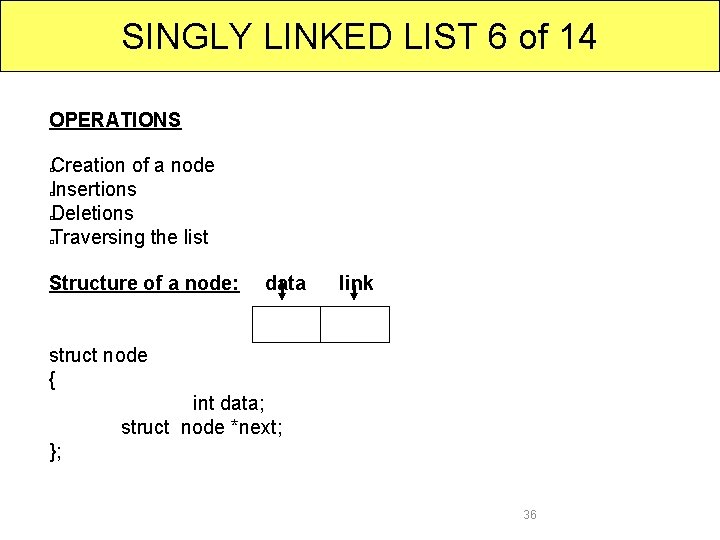
SINGLY LINKED LIST 6 of 14 OPERATIONS Creation of a node Insertions Deletions Traversing the list � � Structure of a node: data link struct node { int data; struct node *next; }; 36

SINGLY LINKED LIST 7 of 14 CREATION OF A NODE: Inittially first=NULL last=NULL struct node *cur; cur=(struct node*)malloc(size of(struct node)); Read cur->data cur->link=NULL 37

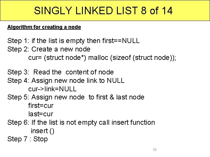
SINGLY LINKED LIST 8 of 14 Algorithm for creating a node Step 1: if the list is empty then first==NULL Step 2: Create a new node cur= (struct node*) malloc (sizeof (struct node)); Step 3: Read the content of node Step 4: Assign new node link to NULL cur->link=NULL Step 5: Assign new node to first & last node first=cur last=cur Step 6: If the list is not empty call insert function insert () Step 7 : Stop 38

SINGLY LINKED LIST 9 of 14 INSERTION: How do we place elements in the list: Usually, there are 4 cases we can use: • at the beginning • at the end of the list • after a given element • before a given element 39

SINGLY LINKED LIST 10 of 14 Case 1 : at the beginning Pseudo code: 1. Inserting at beginning of list. 2. if (first! = NULL) 3. { 4. Cur=(struct node*) malloc (sizeof(struct node)) 5. Read cur->data 6. Cur->lnk=first 7. First=cur 8. } 40

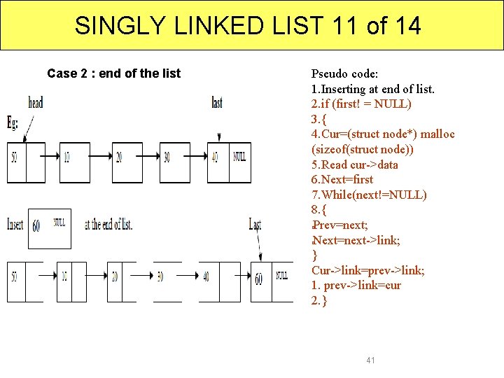
SINGLY LINKED LIST 11 of 14 Case 2 : end of the list Pseudo code: 1. Inserting at end of list. 2. if (first! = NULL) 3. { 4. Cur=(struct node*) malloc (sizeof(struct node)) 5. Read cur->data 6. Next=first 7. While(next!=NULL) 8. { Prev=next; Next=next->link; } Cur->link=prev->link; 1. prev->link=cur 2. } � � 41

SINGLY LINKED LIST 12 of 14 Case 3 : after a given element Pseudo code: 1. Inserting at end of list. 2. if (first! = NULL) 3. { 4. Cur=(struct node*) malloc (sizeof(struct node)) 5. Read cur->data 6. Next=first 7. while(next!=NULL) 8. { 9. if(next->data = = key) 10. break; 11. else 12. next=next->link; 13. } 14. cur -> link = next->link; 15. next->link = cur; 16. } 42

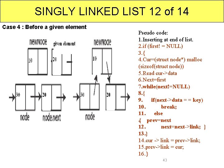
SINGLY LINKED LIST 12 of 14 Case 4 : Before a given element Pseudo code: 1. Inserting at end of list. 2. if (first! = NULL) 3. { 4. Cur=(struct node*) malloc (sizeof(struct node)) 5. Read cur->data 6. Next=first 7. while(next!=NULL) 8. { 9. if(next->data = = key) 10. break; 11. else { prev=next 12. next=next->link; } 13. } 14. cur -> link = prev->link; 15. prev->link = cur; 16. } � 43

SINGLY LINKED LIST 12 of 14 DELETION: Removing an element from the list, without destroying the integrity of the list itself. When we delete a node we logically remove the node from the list by changing links and physically remove it from heap 1)deletion from beginning of list 2)deletion at middle of list 3)deletion at end of list 44

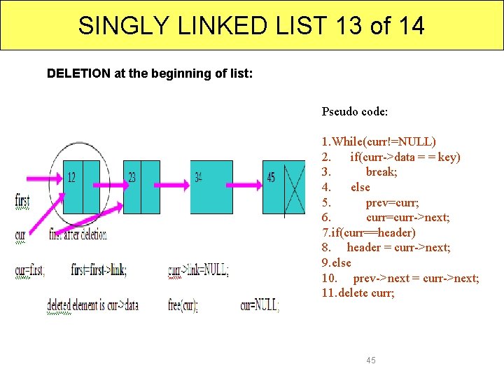
SINGLY LINKED LIST 13 of 14 DELETION at the beginning of list: Pseudo code: 1. While(curr!=NULL) 2. if(curr->data = = key) 3. break; 4. else 5. prev=curr; 6. curr=curr->next; 7. if(curr==header) 8. header = curr->next; 9. else 10. prev->next = curr->next; 11. delete curr; 45

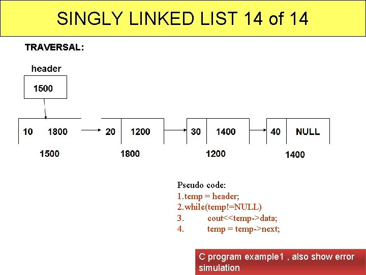
SINGLY LINKED LIST 14 of 14 TRAVERSAL: Pseudo code: 1. temp = header; 2. while(temp!=NULL) 3. cout<<temp->data; 4. temp = temp->next; C program example 1 , also show error 46 simulation

CIRCULARLY LINKED LIST A circularly linked list, or simply circular list, is a linked list in which the last node is always points to the first node. This type of list can be build just by replacing the NULL pointer at the end of the list with a pointer which points to the first node. There is no first or last node in the circular list. Advantages: Any node can be traversed starting from any other node in the list. There is no need of NULL pointer to signal the end of the list and hence, all pointers contain valid addresses. In contrast to singly linked list, deletion operation in circular list is simplified as the search for the previous node of an element to be deleted can be started from that item itself. 47

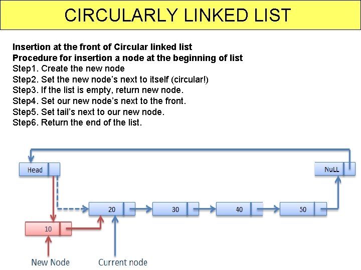
CIRCULARLY LINKED LIST Insertion at the front of Circular linked list Procedure for insertion a node at the beginning of list Step 1. Create the new node Step 2. Set the new node’s next to itself (circular!) Step 3. If the list is empty, return new node. Step 4. Set our new node’s next to the front. Step 5. Set tail’s next to our new node. Step 6. Return the end of the list. 48

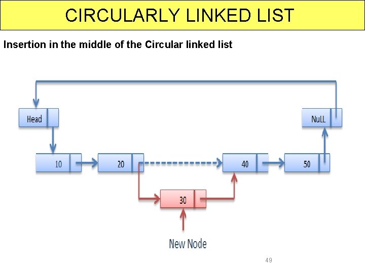
CIRCULARLY LINKED LIST Insertion in the middle of the Circular linked list 49

CIRCULARLY LINKED LIST Insertion at the end of Circular linked list Procedure for insertion a node at the end of list Step 1. Create the new node Step 2. Set the new node’s next to itself (circular!) Step 3. If the list is empty, return new node. Step 4. Set our new node’s next to the front. Step 5. Set tail’s next to our new node. Step 6. Return the end of the list. 50

CIRCULARLY LINKED LIST Deletion In Circular linked list There are three situation for Deleting element in list. 1. Deletion at beginning of the Circular linked list. 2. Deletion at the middle of the Circular linked list. 3. Deletion at the end of the Circular linked list. 51

CIRCULARLY LINKED LIST 1. Deletion at beginning of the Circular linked list. After Deletion 52

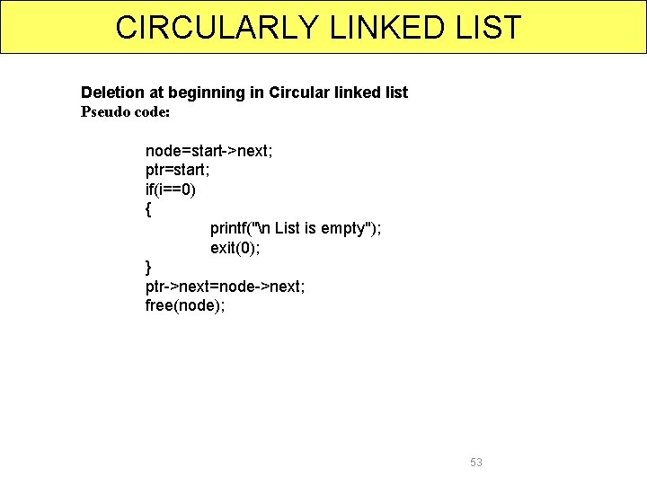
CIRCULARLY LINKED LIST Deletion at beginning in Circular linked list Pseudo code: node=start->next; ptr=start; if(i==0) { printf("n List is empty"); exit(0); } ptr->next=node->next; free(node); 53

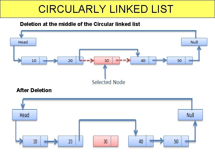
CIRCULARLY LINKED LIST Deletion at the middle of the Circular linked list After Deletion 54

CIRCULARLY LINKED LIST Deletion at location in Circular linked list Pseudo code: if(node_no==delete_no) { ptr->next=node->next; free(node); flag=1; break; } else { ptr=ptr->next; node=node->next; } node_no++; count--; } if(flag==0) { printf("n Position not found"); 55

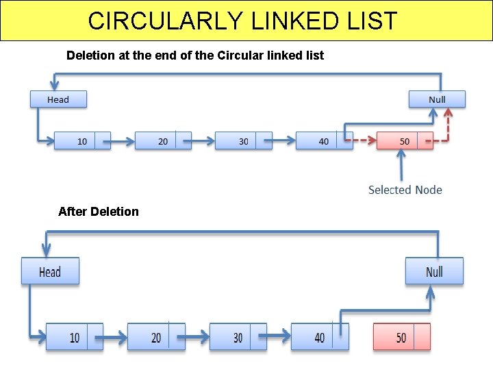
CIRCULARLY LINKED LIST Deletion at the end of the Circular linked list After Deletion 56

CIRCULARLY LINKED LIST Deletion at Last Node Pseudo code: node=start->next; ptr=start; count=i; if(i==0) { printf("n List is empty"); exit(0); } while(count) { node_no++; ptr=ptr->next; node=node->next; count--; } node=start->next; ptr=start; while(node_no!=1) { node_no--; ptr=ptr->next; node=node->next; } if(node_no==1) ptr->next=node->next; free(node); } { 57 C program example: 2 , also show error simulation

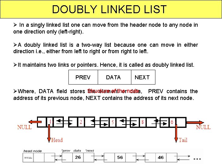
DOUBLY LINKED LIST In a singly linked list one can move from the header node to any node in one direction only (left-right). A doubly linked list is a two-way list because one can move in either direction i. e. , either from left to right or from right to left. It maintains two links or pointers. Hence, it is called as doubly linked list. PREV DATA NEXT Where, DATA field stores Structure of the node the element or data, PREV contains the address of its previous node, NEXT contains the address of its next node. 58

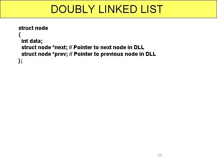
DOUBLY LINKED LIST struct node { int data; struct node *next; // Pointer to next node in DLL struct node *prev; // Pointer to previous node in DLL }; 59

DOUBLY LINKED LIST Advantages over singly linked list 1) A DLL can be traversed in both forward and backward direction. 2) The delete operation in DLL is more efficient if pointer to the node to be deleted is given. In singly linked list, to delete a node, pointer to the previous node is needed. To get this previous node, sometimes the list is traversed. In DLL, we can get the previous node using previous pointer. Disadvantages over singly linked list 1) Every node of DLL Require extra space for an previous pointer. It is possible to implement DLL with single pointer though. 2) All operations require an extra pointer previous to be maintained. For example, in insertion, we need to modify previous pointers together with 60 next pointers. For example in following functions for insertions at different

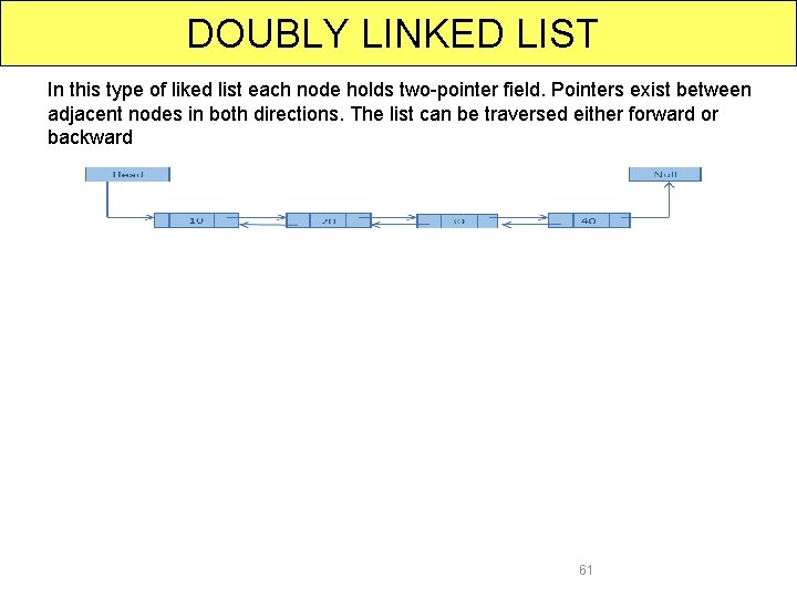
DOUBLY LINKED LIST In this type of liked list each node holds two-pointer field. Pointers exist between adjacent nodes in both directions. The list can be traversed either forward or backward 61

DOUBLY LINKED LIST Creating a New Node Pseudo code: ptr=(node*)malloc(sizeof(node)); ptr->info=item; if(*start==NULL) { ptr->prev = ptr->next = NULL ; *start = *end = ptr ; } else { ptr->prev = *end; (*end)->next = ptr ; ptr->next= NULL; (*end)=ptr; } 62

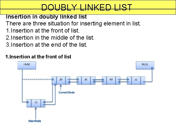
DOUBLY LINKED LIST Insertion in doubly linked list There are three situation for inserting element in list. 1. Insertion at the front of list. 2. Insertion in the middle of the list. 3. Insertion at the end of the list. 1. Insertion at the front of list 63

DOUBLY LINKED LIST Insert at front of the list Pseudo code: ptr=(node*)malloc(sizeof(node)); ptr->info=item; if(*start==NULL) { *start=ptr; *end=ptr; } else { ptr->prev = NULL; ptr->next=*start; (*start)->prev=ptr; *start=ptr; } Algorithm Insert. At. Front. Dll(info, prev, next, start, end) 1. create a new node and address in assigned to ptr. 2. check[overflow] if(ptr=NULL) write: overflow and exit 3. set Info[ptr]=item; 4. if(start=NULL) set prev[ptr] = next[ptr] = NULL set start = end = ptr else set prev[ptr] = NULL next[ptr] = start set prev[start] = ptr set start = ptr [end if] 5. Exit. 64

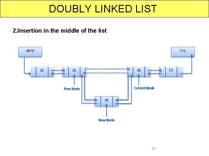
DOUBLY LINKED LIST 2. Insertion in the middle of the list 65

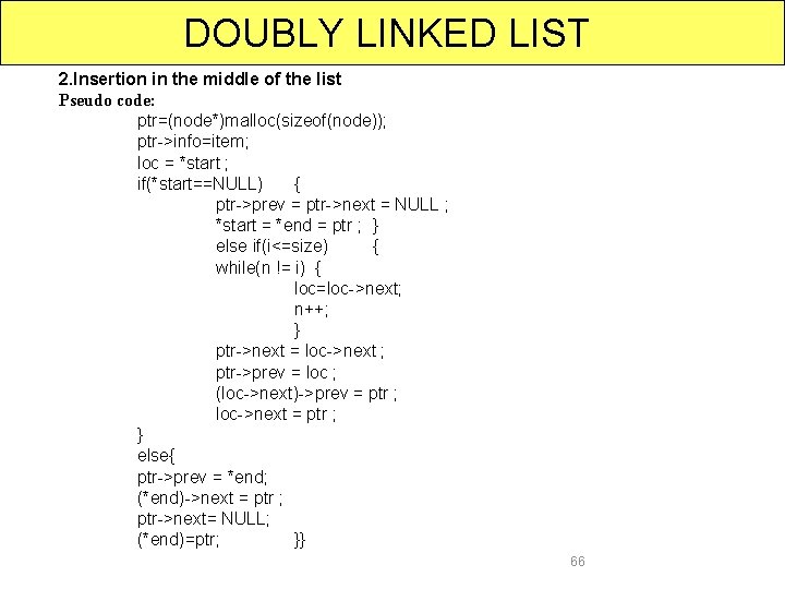
DOUBLY LINKED LIST 2. Insertion in the middle of the list Pseudo code: ptr=(node*)malloc(sizeof(node)); ptr->info=item; loc = *start ; if(*start==NULL) { ptr->prev = ptr->next = NULL ; *start = *end = ptr ; } else if(i<=size) { while(n != i) { loc=loc->next; n++; } ptr->next = loc->next ; ptr->prev = loc ; (loc->next)->prev = ptr ; loc->next = ptr ; } else{ ptr->prev = *end; (*end)->next = ptr ; ptr->next= NULL; (*end)=ptr; }} 66

DOUBLY LINKED LIST 3. Insertion at the end of the list 67

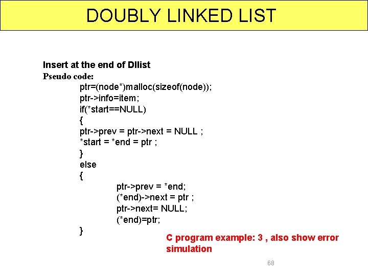
DOUBLY LINKED LIST Insert at the end of Dllist Pseudo code: ptr=(node*)malloc(sizeof(node)); ptr->info=item; if(*start==NULL) { ptr->prev = ptr->next = NULL ; *start = *end = ptr ; } else { ptr->prev = *end; (*end)->next = ptr ; ptr->next= NULL; (*end)=ptr; } C program example: 3 , also show error simulation 68

Representation of single & two dimensional arrays Array Definition: Types: 1 D Array Definition: Declaration: Assigning values: Calling: Example: 2 D Array Definition Declaration: Assigning values: Calling: Example: 69

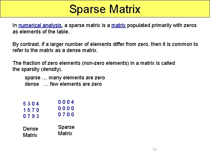
Sparse Matrix In numerical analysis, a sparse matrix is a matrix populated primarily with zeros as elements of the table. By contrast, if a larger number of elements differ from zero, then it is common to refer to the matrix as a dense matrix. The fraction of zero elements (non-zero elements) in a matrix is called the sparsity (density). sparse … many elements are zero dense … few elements are zero 5 3 0 4 0 0 0 0 1 5 7 0 0 0 7 9 3 Dense Matrix Sparse Matrix 70

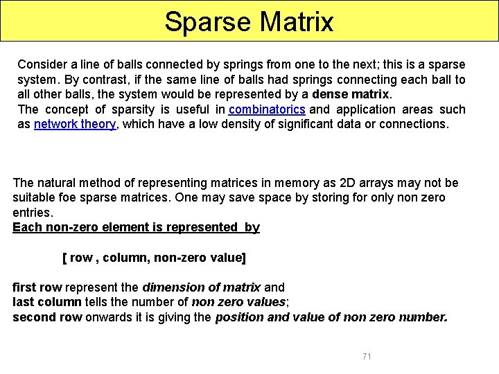
Sparse Matrix Consider a line of balls connected by springs from one to the next; this is a sparse system. By contrast, if the same line of balls had springs connecting each ball to all other balls, the system would be represented by a dense matrix. The concept of sparsity is useful in combinatorics and application areas such as network theory, which have a low density of significant data or connections. The natural method of representing matrices in memory as 2 D arrays may not be suitable foe sparse matrices. One may save space by storing for only non zero entries. Each non-zero element is represented by [ row , column, non-zero value] first row represent the dimension of matrix and last column tells the number of non zero values; second row onwards it is giving the position and value of non zero number. 71

Sparse Matrix Two types of Sparse Matrix Representation 1. Array Representation of Sparse Matrix 1. Linked List Representation of Sparse Matrix 72

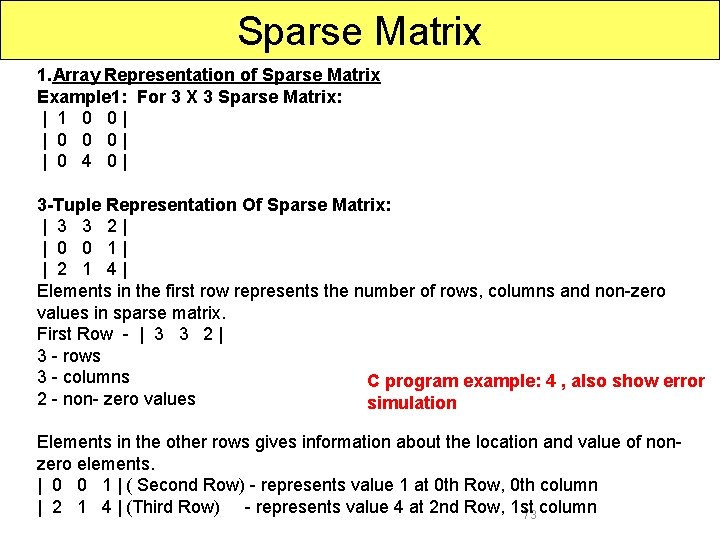
Sparse Matrix 1. Array Representation of Sparse Matrix Example 1: For 3 X 3 Sparse Matrix: | 1 0 0 | | 0 4 0 | 3 -Tuple Representation Of Sparse Matrix: | 3 3 2 | | 0 0 1 | | 2 1 4 | Elements in the first row represents the number of rows, columns and non-zero values in sparse matrix. First Row - | 3 3 2 | 3 - rows 3 - columns C program example: 4 , also show error 2 - non- zero values simulation Elements in the other rows gives information about the location and value of nonzero elements. | 0 0 1 | ( Second Row) - represents value 1 at 0 th Row, 0 th column | 2 1 4 | (Third Row) - represents value 4 at 2 nd Row, 1 st column 73

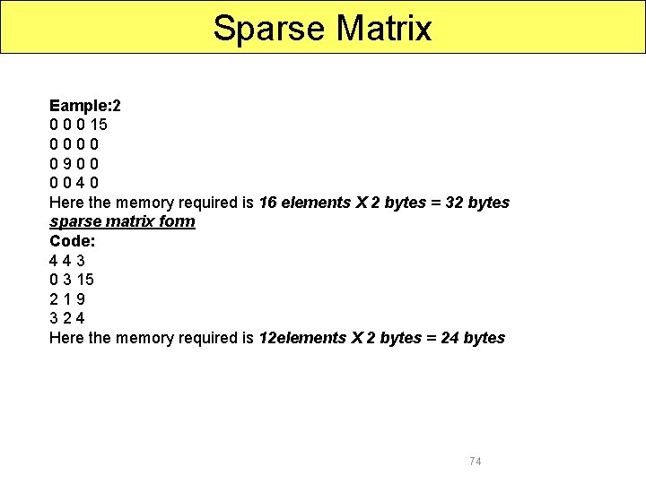
Sparse Matrix Eample: 2 0 0 0 15 0 0 0 9 0 0 4 0 Here the memory required is 16 elements X 2 bytes = 32 bytes sparse matrix form Code: 4 4 3 0 3 15 2 1 9 3 2 4 Here the memory required is 12 elements X 2 bytes = 24 bytes 74

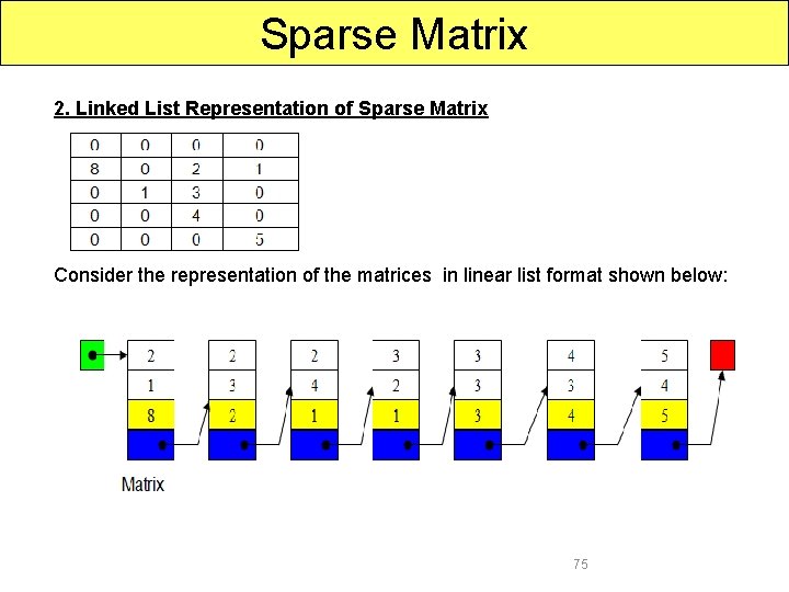
Sparse Matrix 2. Linked List Representation of Sparse Matrix Consider the representation of the matrices in linear list format shown below: 75

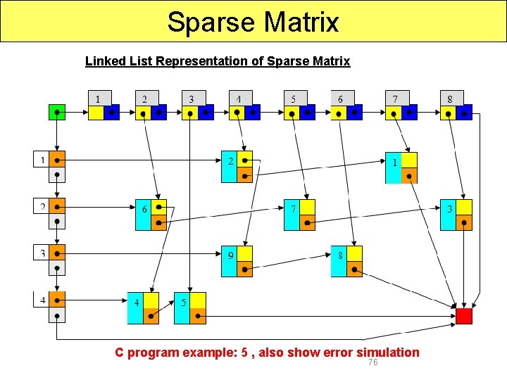
Sparse Matrix Linked List Representation of Sparse Matrix C program example: 5 , also show error simulation 76

End 77