UNIT1 INTRODUCTION Introduction u Signal something conveys information

UNIT-1 INTRODUCTION

Introduction u Signal: something conveys information u Signals are represented mathematically as functions of one or more independent variables. u Continuous-time (analog) signals, discrete-time signals, digital signals u Signal-processing systems are classified along the same lines as signals: Continuous-time (analog) systems, discrete-time systems, digital systems u Discrete-time signal u Sampling a continuous-time signal u Generated directly by some discrete-time process

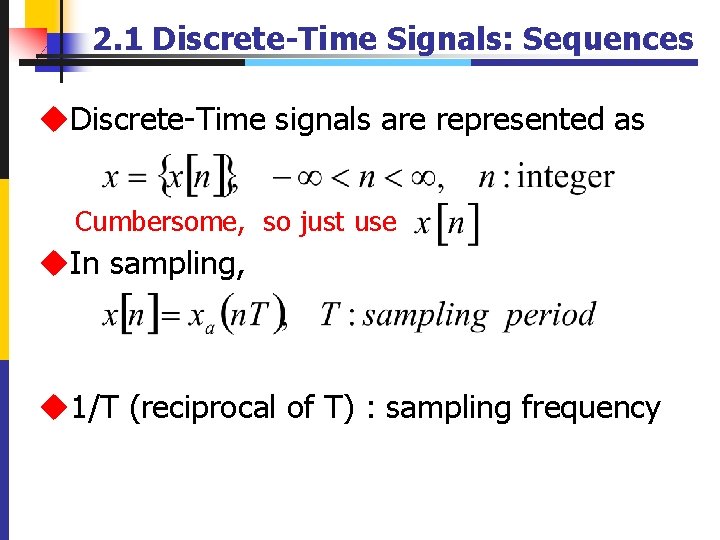
2. 1 Discrete-Time Signals: Sequences u. Discrete-Time signals are represented as Cumbersome, so just use u. In sampling, u 1/T (reciprocal of T) : sampling frequency

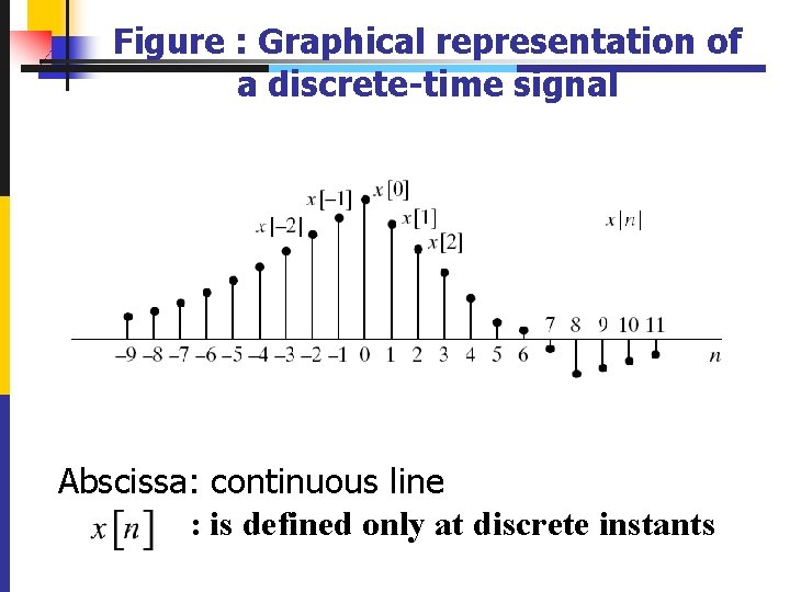
Figure : Graphical representation of a discrete-time signal Abscissa: continuous line : is defined only at discrete instants

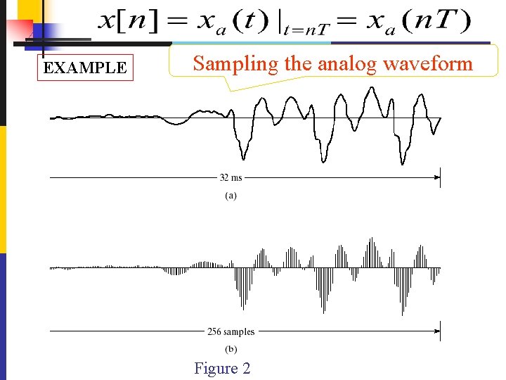
EXAMPLE Sampling the analog waveform Figure 2

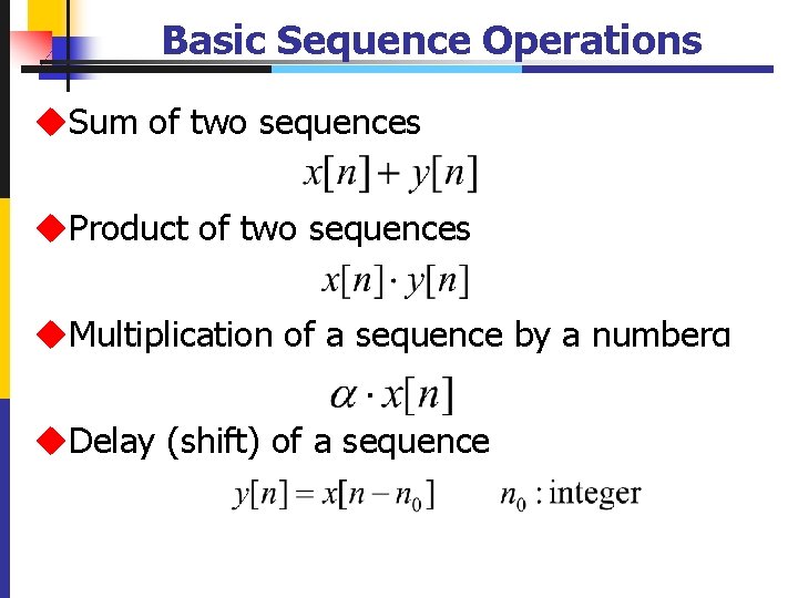
Basic Sequence Operations u. Sum of two sequences u. Product of two sequences u. Multiplication of a sequence by a numberα u. Delay (shift) of a sequence

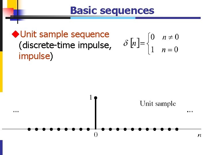
Basic sequences u. Unit sample sequence (discrete-time impulse, impulse)

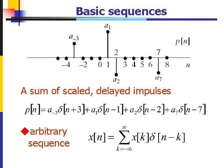
Basic sequences A sum of scaled, delayed impulses uarbitrary sequence

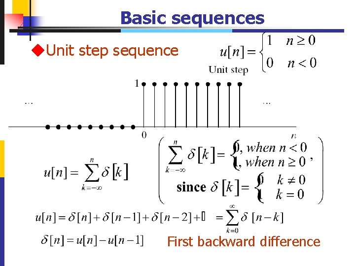
Basic sequences u. Unit step sequence First backward difference

Basic Sequences u. Exponential sequences u. A and α are real: x[n] is real u. A is positive and 0<α<1, x[n] is positive and decrease with increasing n u-1<α<0, x[n] alternate in sign, but decrease in magnitude with increasing n u : x[n] grows in magnitude as n increases 6/9/2021

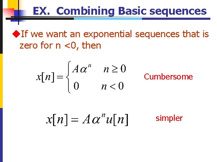
EX. Combining Basic sequences u. If we want an exponential sequences that is zero for n <0, then Cumbersome simpler 11

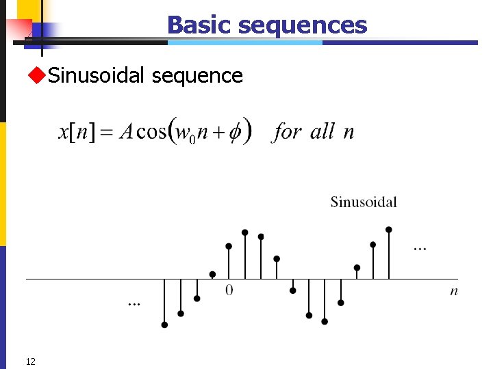
Basic sequences u. Sinusoidal sequence 12

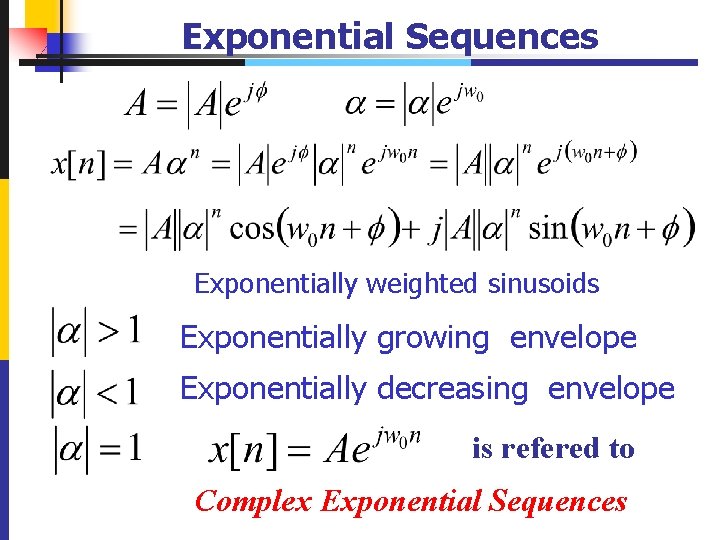
Exponential Sequences Exponentially weighted sinusoids Exponentially growing envelope Exponentially decreasing envelope is refered to Complex Exponential Sequences 13

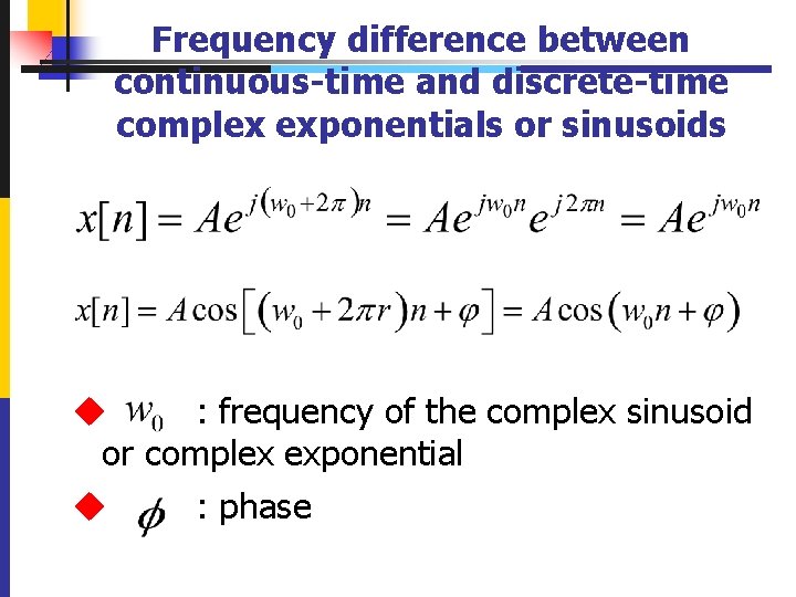
Frequency difference between continuous-time and discrete-time complex exponentials or sinusoids u : frequency of the complex sinusoid or complex exponential u : phase

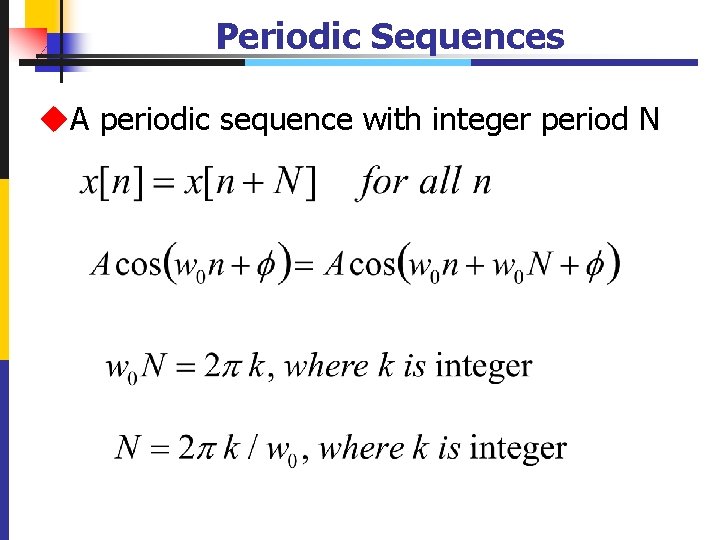
Periodic Sequences u. A periodic sequence with integer period N

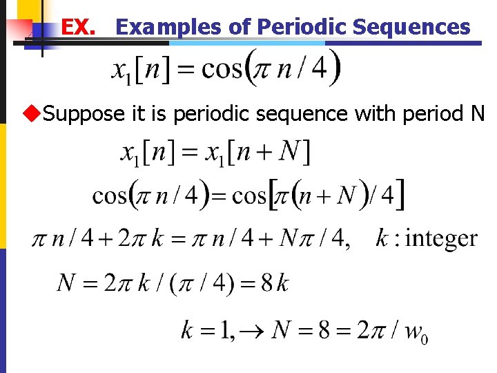
EX. Examples of Periodic Sequences u. Suppose it is periodic sequence with period N 16

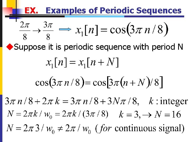
EX. Examples of Periodic Sequences u. Suppose it is periodic sequence with period N

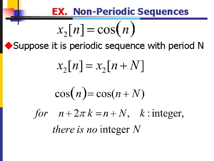
EX. Non-Periodic Sequences u. Suppose it is periodic sequence with period N

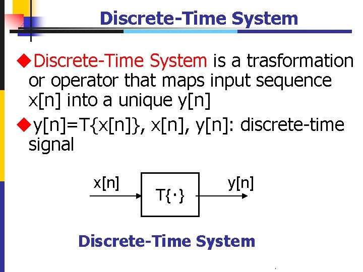
Discrete-Time System u. Discrete-Time System is a trasformation or operator that maps input sequence x[n] into a unique y[n] uy[n]=T{x[n]}, x[n], y[n]: discrete-time signal x[n] T{‧} y[n] Discrete-Time System.

Properties of Discrete-time systems Memoryless (memory) system u. Memoryless systems: the output y[n] at every value of n depends only on the input x[n] at the same value of n 20

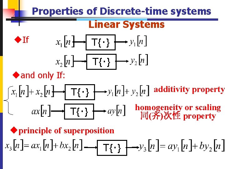
Properties of Discrete-time systems Linear Systems u. If T{‧} uand only If: additivity property T{‧} homogeneity or scaling 同(齐)次性 property T{‧} uprinciple of superposition T{‧} 21

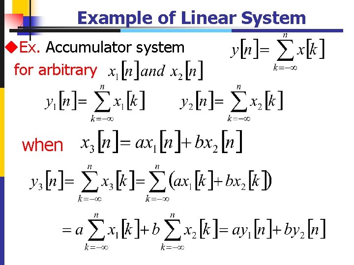
Example of Linear System u. Ex. Accumulator system for arbitrary when 22

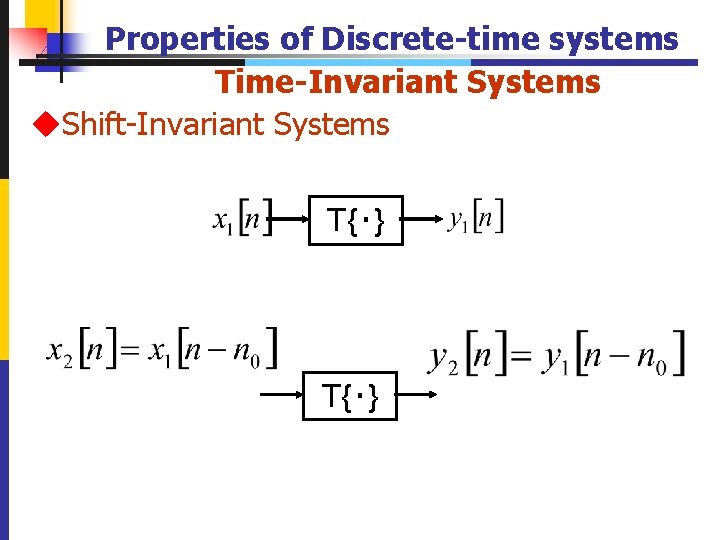
Properties of Discrete-time systems Time-Invariant Systems u. Shift-Invariant Systems T{‧} 23

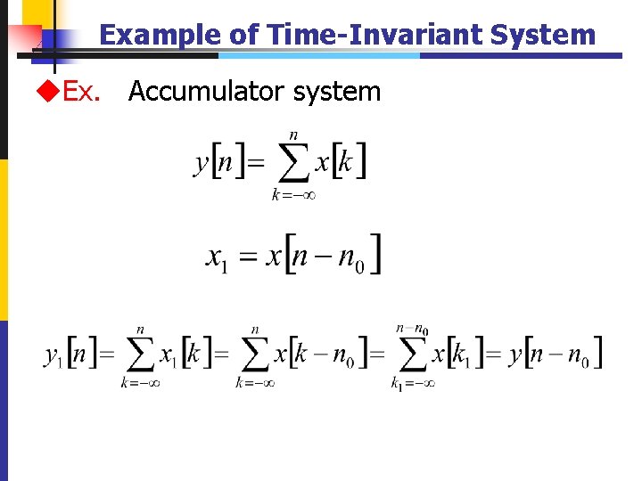
Example of Time-Invariant System u. Ex. Accumulator system 24

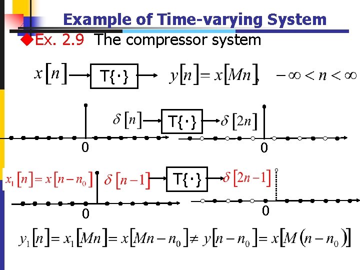
Example of Time-varying System u. Ex. 2. 9 The compressor system T{‧} 0 0 T{‧} 0 25 0

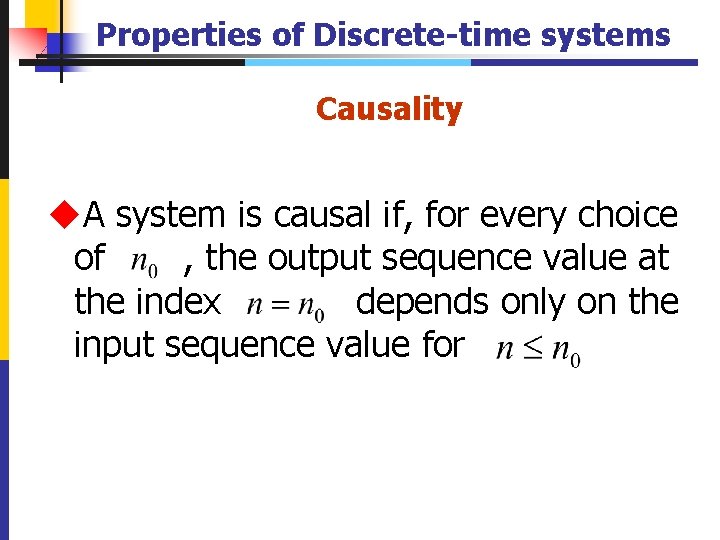
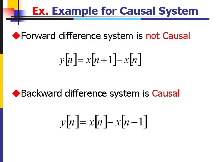
Properties of Discrete-time systems Causality u. A system is causal if, for every choice of , the output sequence value at the index depends only on the input sequence value for 26

Ex. Example for Causal System u. Forward difference system is not Causal u. Backward difference system is Causal 27

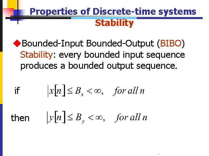
Properties of Discrete-time systems Stability u. Bounded-Input Bounded-Output (BIBO) Stability: every bounded input sequence produces a bounded output sequence. if then 28 .

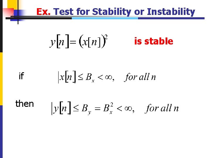
Ex. Test for Stability or Instability is stable if then 29

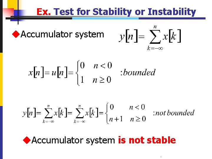
Ex. Test for Stability or Instability u. Accumulator system is not stable 30 .

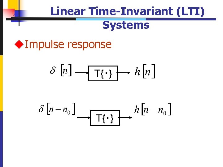
Linear Time-Invariant (LTI) Systems u. Impulse response T{‧} 31

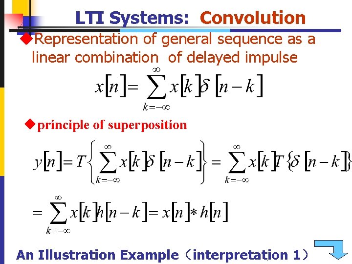
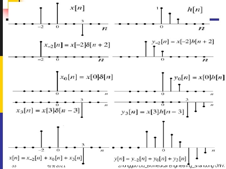
LTI Systems: Convolution u. Representation of general sequence as a linear combination of delayed impulse uprinciple of superposition An Illustration Example（interpretation 1）. 32

33 6/9/2021 Zhongguo Liu_Biomedical Engineering_Shandong Univ.

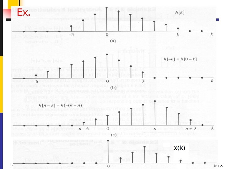
Computation of the Convolution （interpretation 2） ureflecting h[k] about the origion to obtain h[-k] u. Shifting the origin of the reflected sequence to k=n 34 .

Ex. 35 6/9/2021 Zhongguo Liu_Biomedical Engineering_Shandong Univ.

Convolution can be realized by –Reflecting h[k] about the origin to obtain h[-k]. –Shifting the origin of the reflected sequences to k=n. –Computing the weighted moving average of x[k] by using the weights given by h[n-k]. 36

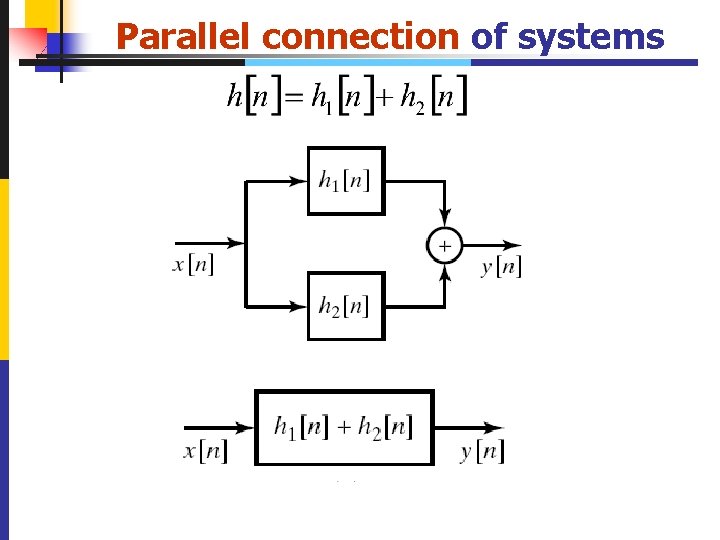
Properties of LTI Systems u. Convolution is commutative(可交换的) x[n] h[n] y[n] h[n] x[n] y[n] u. Convolution is distributed over addition 37

Cascade connection of systems x [ n] h 1[ n] h 2[ n] y [ n] x [ n] h 2[ n] h 1[ n] y [ n] x [ n] 38 h 1[n] ] h 2[n] y [ n]

Parallel connection of systems 39

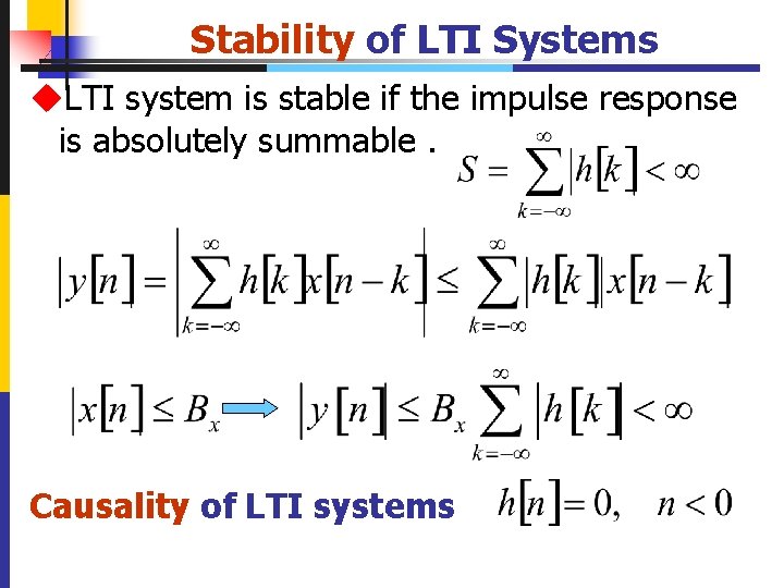
Stability of LTI Systems u. LTI system is stable if the impulse response is absolutely summable. Causality of LTI systems 40

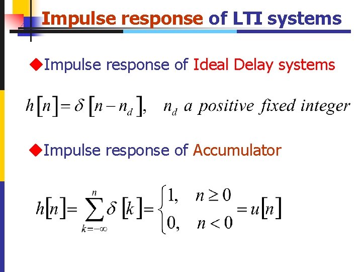
Impulse response of LTI systems u. Impulse response of Ideal Delay systems u. Impulse response of Accumulator 41

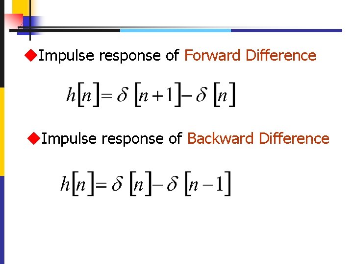
u. Impulse response of Forward Difference u. Impulse response of Backward Difference 42

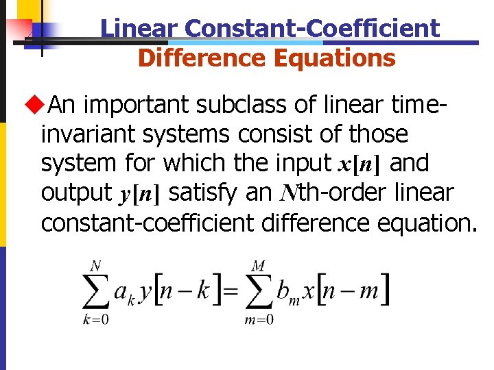
Linear Constant-Coefficient Difference Equations u. An important subclass of linear timeinvariant systems consist of those system for which the input x[n] and output y[n] satisfy an Nth-order linear constant-coefficient difference equation. 43

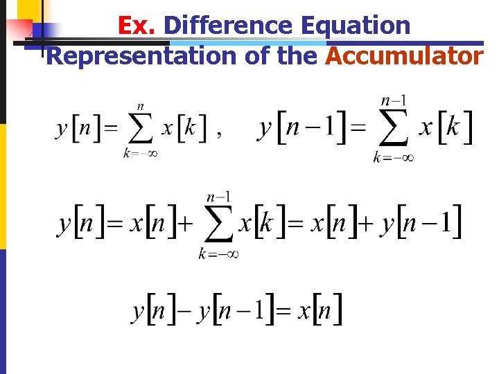
Ex. Difference Equation Representation of the Accumulator 44

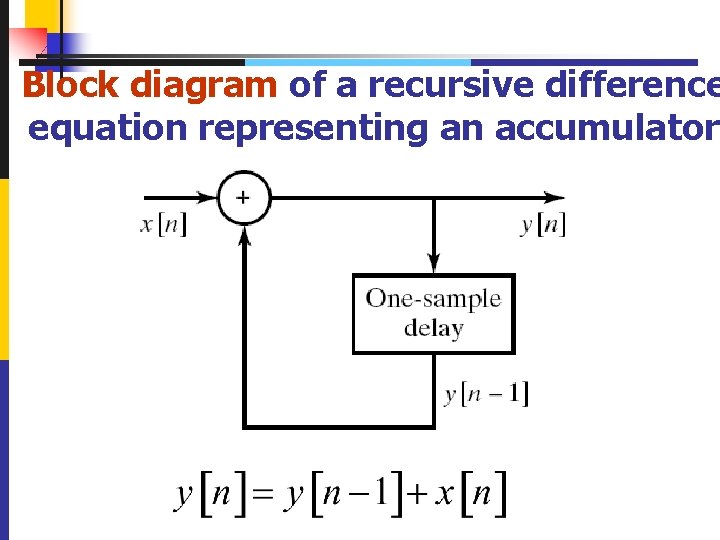
Block diagram of a recursive difference equation representing an accumulator 45

Difference Equation Representation of the System u. An unlimited number of distinct difference equations can be used to represent a given linear time-invariant input-output relation. 46

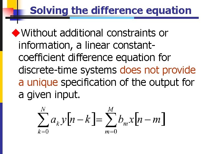
Solving the difference equation u. Without additional constraints or information, a linear constantcoefficient difference equation for discrete-time systems does not provide a unique specification of the output for a given input. 47

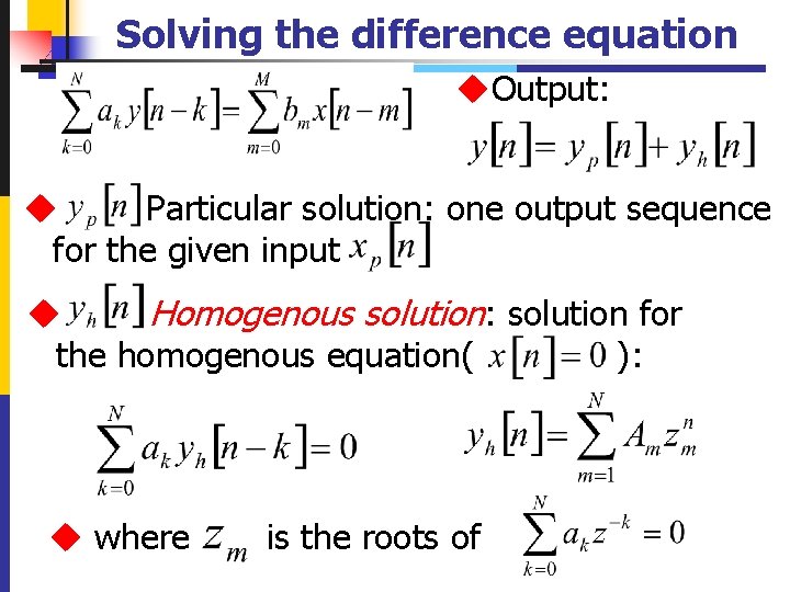
Solving the difference equation u. Output: u Particular solution: one output sequence for the given input u Homogenous solution: solution for the homogenous equation( ): u where 48 is the roots of

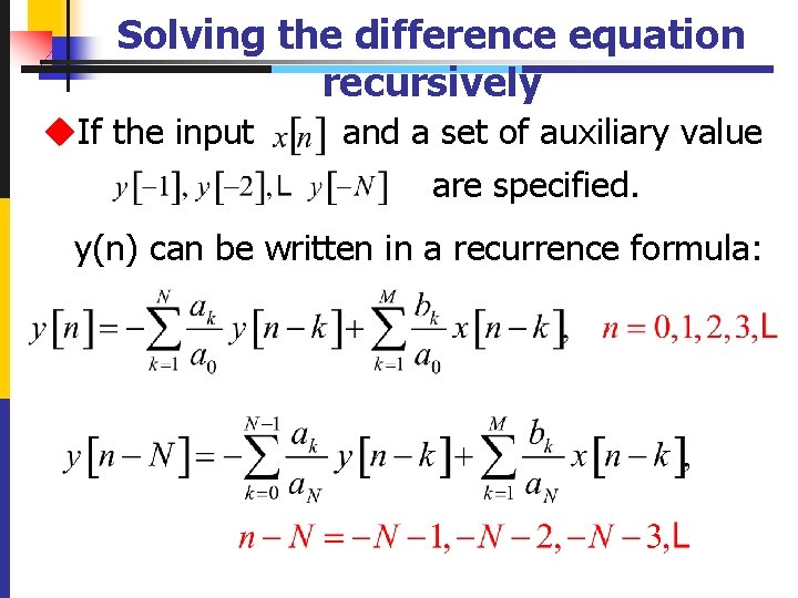
Solving the difference equation recursively u. If the input and a set of auxiliary value are specified. y(n) can be written in a recurrence formula: 49

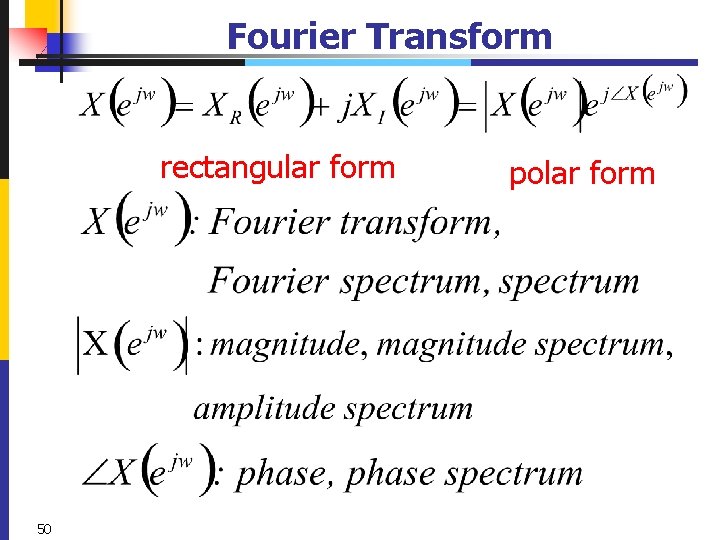
Fourier Transform rectangular form 50 polar form

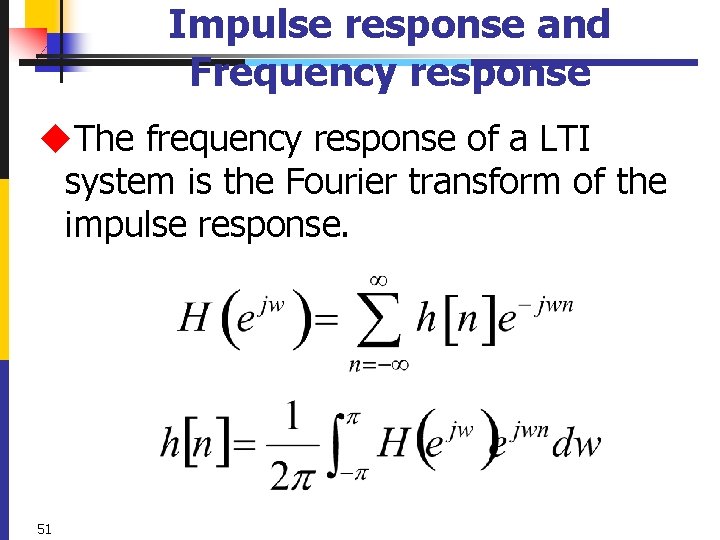
Impulse response and Frequency response u. The frequency response of a LTI system is the Fourier transform of the impulse response. 51

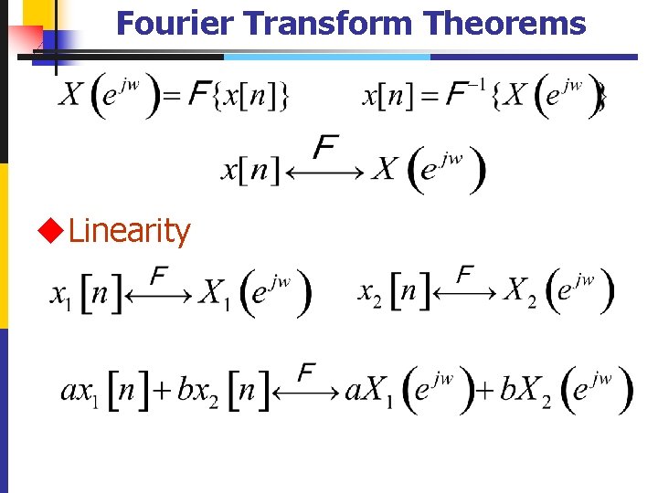
Fourier Transform Theorems u. Linearity 52

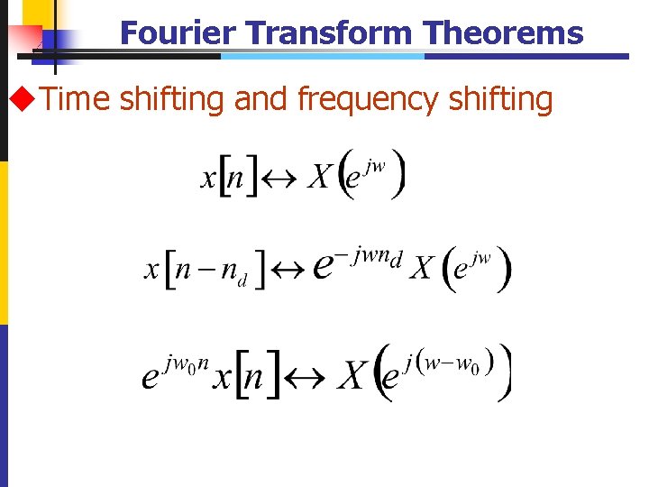
Fourier Transform Theorems u. Time shifting and frequency shifting

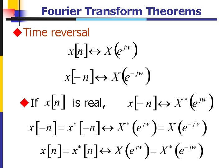
Fourier Transform Theorems u. Time reversal u. If is real,

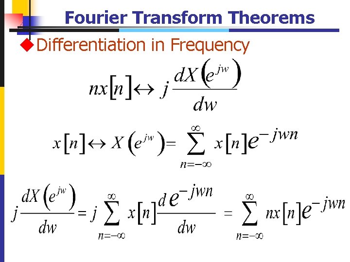
Fourier Transform Theorems u. Differentiation in Frequency 55

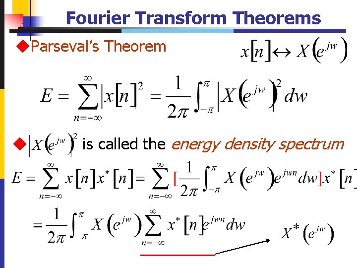
Fourier Transform Theorems u. Parseval’s Theorem u is called the energy density spectrum

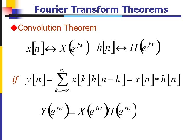
Fourier Transform Theorems u. Convolution Theorem if

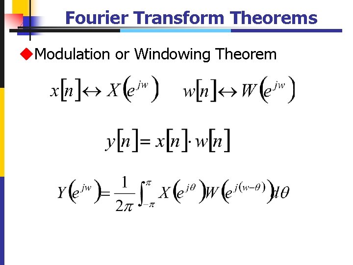
Fourier Transform Theorems u. Modulation or Windowing Theorem