UNIT IV INPUT and OUTPUT Devices Remote Sensing

UNIT IV INPUT and OUTPUT Devices Remote Sensing and GIS

DATA INPUT TECHNIQUES • Since the input of attribute data is usually quite simple, the discussion of data input techniques will be limited to spatial data only. There is no single method of entering the spatial data into a GIS. Rather, there are several, mutually compatible methods that can be used singly or in combination. • The choice of data input method is governed largely by the application, the available budget, and the type and the complexity of data being input. • There at least four basic procedures for inputting spatial data into a GIS. These are: – – Manual digitizing; Automatic scanning; Entry of coordinates using coordinate geometry; and the Conversion of existing digital data.

Digitizing • Digitizing can be done in a point mode, where single points are recorded one at a time, or in a stream mode, where a point is collected on regular intervals of time or distance, measured by an X and Y movement, e. g. every 3 metres. Digitizing can also be done blindly or with a graphics terminal. Blind digitizing infers that the graphic result is not immediately viewable to the person digitizing. Most systems display the digitized linework as it is being digitized on an accompanying graphics terminal. • Most GIS's use a spaghetti mode of digitizing. This allows the user to simply digitize lines by indicating a start point and an end point. Data can be captured in point or stream mode. However, some systems do allow the user to capture the data in an arc/node topological data structure. The arc/node data structure requires that the digitizer identify nodes.

Manual digitizing has many advantages. • These include: – Low capital cost, e. g. digitizing tables are cheap; – Low cost of labour; – Flexibility and adaptability to different data types and sources; – Easily taught in a short amount of time - an easily mastered skill – Generally the quality of data is high; – Digitizing devices are very reliable and most often offer a greater precision that the data warrants; and – Ability to easily register and update existing data.

Automatic Scanning • Scanners are generally expensive to acquire and operate. As well, most scanning devices have limitations with respect to the capture of selected features, e. g. text and symbol recognition. Experience has shown that most scanned data requires a substantial amount of manual editing to create a clean data layer.

• Given these basic constraints some other practical limitations of scanners should be identified. These include: – hard copy maps are often unable to be removed to where a scanning device is available, e. g. most companies or agencies cannot afford their own scanning device and therefore must send their maps to a private firm for scanning; – hard copy data may not be in a form that is viable for effective scanning, e. g. maps are of poor quality, or are in poor condition; – geographic features may be too few on a single map to make it practical, cost-justifiable, to scan; – often on busy maps a scanner may be unable to distinguish the features to be captured from the surrounding graphic information, e. g. dense contours with labels; – with raster scanning there it is difficult to read unique labels (text) for a geographic feature effectively; and – scanning is much more expensive than manual digitizing, considering all the cost/performance issues.

DATA EDITING AND QUALITY ASSURANCE • Data editing and verification is in response to the errors that arise during the encoding of spatial and non-spatial data. • The editing of spatial data is a time consuming, interactive process that can take as long, if not longer, than the data input process itself.

• Several kinds of errors can occur during data input. They can be classified as: – Incompleteness of the spatial data. This includes missing points, line segments, and/or polygons. – Locational placement errors of spatial data. These types of errors usually are the result of careless digitizing or poor quality of the original data source. – Distortion of the spatial data. This kind of error is usually caused by base maps that are not scale-correct over the whole image, e. g. aerial photographs, or from material stretch, e. g. paper documents. – Incorrect linkages between spatial and attribute data. This type of error is commonly the result of incorrect unique identifiers (labels) being assigned during manual key in or digitizing. This may involve the assigning of an entirely wrong label to a feature, or more than one label being assigned to a feature. – Attribute data is wrong or incomplete. Often the attribute data does not match exactly with the spatial data. This is because they are frequently from independent sources and often different time periods. Missing data records or too many data records are the most common problems.

• The identification of errors in spatial and attribute data is often difficult. Most spatial errors become evident during the topological building process. • The use of check plots to clearly determine where spatial errors exist is a common practice. • Most topological building functions in GIS software clearly identify the geographic location of the error and indicate the nature of the problem. • Comprehensive GIS software allows users to graphically walk through and edit the spatial errors. Others merely identify the type and coordinates of the error. • Since this is often a labour intensive and time consuming process, users should consider the error correction capabilities very important during the evaluation of GIS software offerings.

Spatial Data Errors • Digitizing allows a user to trace spatial data from a hard copy product, e. g. a map, and have it recorded by the computer software. • Most GIS software has utilities to clean the data and build a topologic structure. If the data is unclean to start with, for whatever reason, the cleaning process can be very lengthy. Interactive editing of data is a distinct reality in the data input process. • The most common problems that occur in converting data into a topological structure include: – slivers and gaps in the line work; – dead ends, e. g. also called dangling arcs, resulting from overshoots and undershoots in the line work; and – bow ties or weird polygons from inappropriate closing of connecting features.

Slivers • Slivers are the most common problem when cleaning data. Slivers frequently occur when coincident boundaries are digitized separately, e. g. once each for adjacent forest stands, once for a lake and once for the stand boundary, or after polygon overlay. • Slivers often appear when combining data from different sources, e. g. forest inventory, soils, and hydrography. It is advisable to digitize data layers with respect to an existing data layer, e. g. hydrography, rather than attempting to match data layers later. • A proper plan and definition of priorities for inputting data layers will save many hours of interactive editing and cleaning.

Dead ends and bow ties or weird polygons • Dead ends usually occur when data has been digitized in a spaghetti mode, or without snapping to existing nodes. • Most GIS software will clean up undershoots and overshoots based on a user defined tolerance, e. g. distance. • The definition of an inappropriate distance often leads to the formation of bow ties or weird polygons during topological building. • Tolerances that are too large will force arcs to snap one another that should not be connected. The result is small polygons called bow ties. • The definition of a proper tolerance for cleaning requires an understanding of the scale and accuracy of the data set.

Attribute Data Errors • • • The identification of attribute data errors is usually not as simple as spatial errors. This is especially true if these errors are attributed to the quality or reliability of the data. Errors as such usually do not surface until later on in the GIS processing. Solutions to these type of problems are much more complex and often do not exist entirely. It is much more difficult to spot errors in attribute data when the values are syntactically good, but incorrect. Data Verification Six clear steps stand out in the data editing and verification process for spatial data. These are: – Visual review. This is usually by check plotting. – Cleanup of lines and junctions. This process is usually done by software first and interactive editing second. – Weeding of excess coordinates. This process involves the removal of redundant vertices by the software for linear and/or polygonal features. – Correction for distortion and warping. Most GIS software has functions for scale correction and rubber sheeting. However, the distinct rubber sheet algorithm used will vary depending on the spatial data model, vector or raster, employed by the GIS. Some raster techniques may be more intensive than vector based algorithms. – Construction of polygons. Since the majority of data used in GIS is polygonal, the construction of polygon features from lines/arcs is necessary. Usually this is done in conjunction with the topological building process. – The addition of unique identifiers or labels. Often this process is manual. However, some systems do provide the capability to automatically build labels for a data layer.

Introduction to Output Devices Output from GIS does not have to be a map. In fact, many GIS are designed with poor map output capabilities Types of output • text - tables, lists, numbers or text in response to query • graphic - maps, screen displays, graphs, perspective plots • digital data - on disk, tape or transmitted across a network • other, not yet common – computer-generated sound – 3 D images

TEXT OUTPUT • perhaps more important than maps for reporting results of analysis • results might be a list or table of selected objects with attributes • queries might result in numerical results, e. g. totals, distances, areas, counts • text output might be delivered by voice generator, e. g. navigation instructions Tables • e. g. list of all cuttable areas of timber, giving area, species, age, estimate of yield in board feet • list is not of great value without an accompanying map to identify each object in the list • examples of specialized lists: – personalized letter to be mailed to all households within 500 m of a planned expressway – list of all hazardous materials stored within 100 m of a fire, transmitted by FAX to fire truck – driving directions for a garbage collection route – work order and accompanying map and marked travel route for each service vehicle operated by utility company, giving day's work locations, nature of work – list and accompanying map of all city voting precincts ranked by degree of support for party in last election

GRAPHIC OUTPUT Graphics peripherals • provide graphic input and output of maps, diagrams and charts • interactive graphics devices allow users to point to objects and identify them in their correct spatial context • an early interactive version of the Space War computer game, developed at MIT in the early 1960 s, ran on a PDP-1 computer using video displays • television-like terminals became common in the early 1960's, and are now the most common way users interact with computer systems • in the next few sections we look at devices for graphic output and the ways their development has influenced GIS • costs are approximate, correct to order of magnitude only

• Raster and vector devices • graphic output devices can be classified into raster and vector groups • raster devices build a picture by filling it with uniform picture elements, usually in rows – e. g. line printers, dot matrix printers, scanners, most CRT terminals – the elements of the picture are called pixels or pels – resolution is sometimes expressed in megapels (approximately equal to 106 pixels) 640 x 480 pixel resolution is 0. 3 megapels; 1280 x 1024 is 1. 3 megapels • vector devices build a picture by drawing lines, shading areas etc. – e. g. plotters, storage tube CRT technology • a raster device may be driven by vector commands, which it then converts for display, and vice versa • conversion between raster and vector may thus occur at several points in a GIS between input and output

HARDCOPY OUTPUT Line printers • the first common device for computer output, cost $30, 000 • capable of printing 200 -1, 000 lines of text per minute • each line composed of 132 characters in fixed positions • entire line printed simultaneously by impact of hammers on ink ribbon • limited set of printable characters • image must be created row by row from the top • most useful for repeated mapping of statistics on a constant base, e. g. census atlas, weekly reports of crime statistics Drawbacks for graphical output because: – – – rectangular cells resolution is fixed, e. g. 1/6 inch by 1/10 inch (4. 2 mm by 2. 5 mm) fixed cell location only limited set of characters can be printed difficult to draw continuous lines

Dot matrix • image composed of rows of dots - often printed in blocks, e. g. 9 or 25 rows at a time • to create shades of grey, control the fraction of dots which are printed in any small area • early versions used hammers on ribbons for each dot - cost $500 • more recent versions use lasers and xerography technology, resolutions up to 300 dots per inch - cost $2, 000 • color versions are available - squirt ink from jets of three or four primary colors - cost $2, 000 • electrostatic plotters use rows of dots, create images of map size - cost $40, 000

Pen plotters • create images by moving a pen under computer control • most are incremental - draw a line using large numbers of movements of fixed size in fixed directions – many have two motors, one for x and one for y • get diagonal movement in only eight directions by using combinations of one or both motors • however, step size is so small that lines appear to go equally easily in all directions • diagram • from a GIS perspective, an important advantage is the ability to plot on top of pre-printed base maps – this avoids having to have all of the base map information in digital form

Types of plotters • lowest cost - $2, 000 - are desktop size, take standard A 4 or similar paper – paper is flat – pens can be changed automatically to generate different colors • mid-range - $25, 000 - are map size paper rolls over drum movement of pen is parallel to axis of drum second direction of movement is by rotating drum problems keeping paper in registration since it may move and stretch during construction of the map/graphic – problems keeping pens moist during long plotting jobs – typical plot jobs can last 3 to 6 hours – – • top range - $100, 000 are high precision – used for drafting, map production – usually flat (&QUOT flatbed"), medium held on exactly flat surface – pen may be replaced by cutting tool on scribe coat

Optical scanners • output on photographic paper • paper mounted on inside of a rotating drum • image created in helical fashion by rotating drum and moving light source along axis of drum • common output devices for remote sensing, image processing

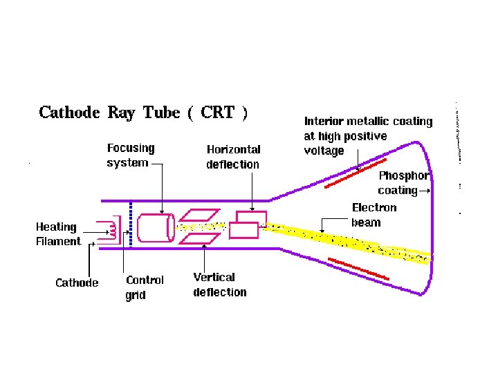
CRTS (CATHODE RAY TUBES) • earliest (ca. 1968) could display rows of characters in fixed positions, little use for showing maps or images • Storage tube technology • Tektronix introduced terminals based on storage tube technology ca. 1970 – major breakthrough in low-cost graphic display ($5, 000) – images drawn by moving electron beam over screen under computer control – image is permanent, not refreshed, so must be erased completely - no selective deletion possible