Unit IV Cost estimation Documentation Prof Prasad Mahale

Unit - IV Cost estimation & Documentation - Prof. Prasad Mahale

GOOD ESTIMATES • Prediction is one that guide us for decision making through out the life cycle. • Prediction is useful only if it is reasonably (practically) accurate. • We do not expect our prediction to be exact, but we expect them to be close to actuals • Record the actual completion times of large number of projects, trying to implement same set of requirements.

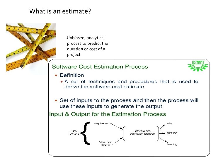
GOOD ESTIMATES What is an estimate? ü We think prediction as a range or window, rather than a single number ü Estimate/prediction is not a target rather an estimate is a probabilistic assessment, so that the value produced by estimate is really the center of a range. ü According to Demarco Estimation is a prediction that is equally likely to be above/below actual result ü Estimate define as median of unknown distribution where it divides the arc under the curve into two equal parts A & B. In other words Actual value is just as likely to be less/greater than estimate

GOOD ESTIMATES What is an estimate?

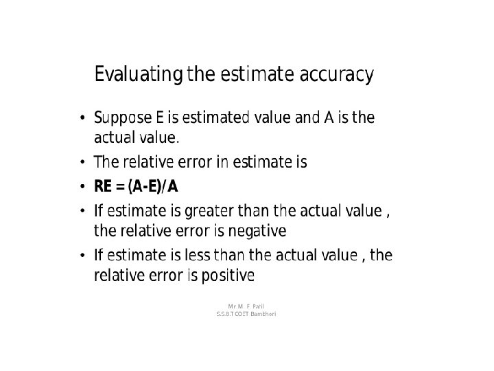
GOOD ESTIMATES Evaluating estimate accuracy: • Once our project is ongoing, we compare actual value with estimate • E- estimate value, A – actual value then relative error in estimate is • Computed as • RE must be positive or negative depending upon values of A & E • Mean Relative Error for n projects is computed to be: • We need to define magnitude of relative error as a absolute value of RE & denoted as MRE. • Then for set of n projects, mean magnitude of relative error is:

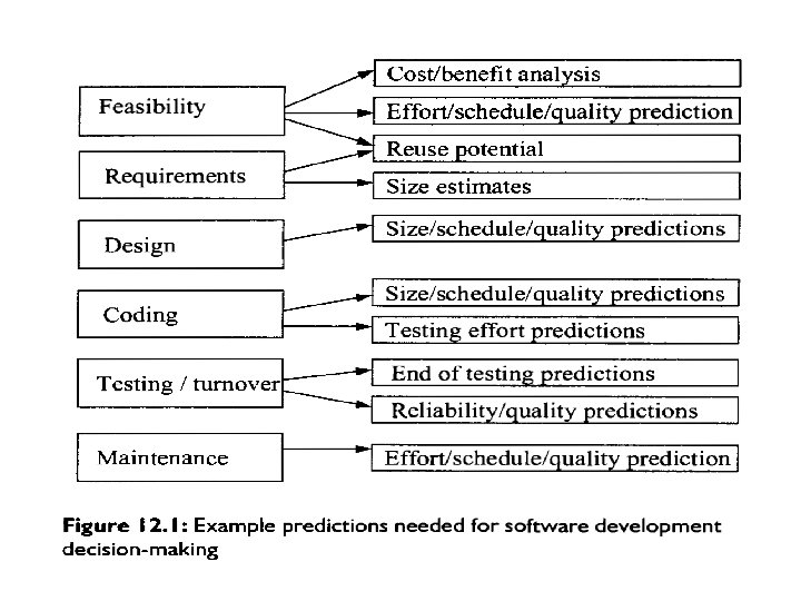
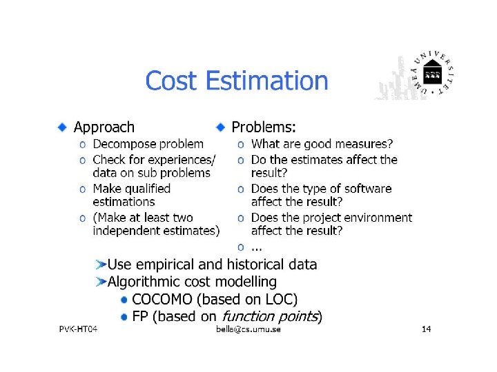
7. COST ESTIMATION : PROBLEM & APPROACHES • Prediction of likely amount of effort , time & staffing level required to build a s/w system • Cost estimation/effort estimation use interchangeably • Cost estimation needed throughout life cycle-determine whether a project is feasible in terms of cost –benefit analysis • Preliminary estimation are difficult to obtain & inaccurate • Prediction support planning & resource planning

7. COST ESTIMATION : PROBLEM & APPROACHES Problem with cost estimation: ü Profession ü Novelty of Application ü Political Problems ü Technical problem Ø 4 -approaches of cost effort & schedule estimation 1. 2. 3. 4. Expert opinion Analogy Decomposition models

7. COST ESTIMATION : PROBLEM & APPROACHES Problems with Cost Estimation ü Profession: it takes advantages of repeatability of their task ü Novelty of Application introduces more uncertainty in prediction ü Political Problems: Manager converts estimation into targets or manipulates estimation parameter to fit into already defined outcomes ü Technical problem: Since we are not encourage to collect data about process and product so very few historical records are available for prediction. • Organization spending more effort & time for estimation in early phases of project and giving less effort after project completion

COST ESTIMATION : PROBLEM & APPROACHES Current Approaches to Cost Estimation 1. Expert opinion 2. Analogy 3. Decomposition 4. models

1. Expert opinion: - - by mature developer’s personal experience Manager describes parameter of project, expert make prediction based on experience Expert may use tools, models or other method for estimation, but not visible to requester Strength relies on quality of expert & experience 2. Analogy: - Estimate compare proposed project with one/more past projects Identify similarity & difference Describe a project in terms of key characteristics Analysis is documented

3. Decomposition: - More thorough analysis Focus on product deliver or task require to build s/w describe in terms of smallest component Activities are decomposed into low-level tasks & estimate are made low-level estimate are combine to produce a complete project estimate 4. Models: - Identify key attributes to effort, generate mathematical formulae - take i/p as experience of developer, implement Language, degree of reuse - I/p value may require decomposition

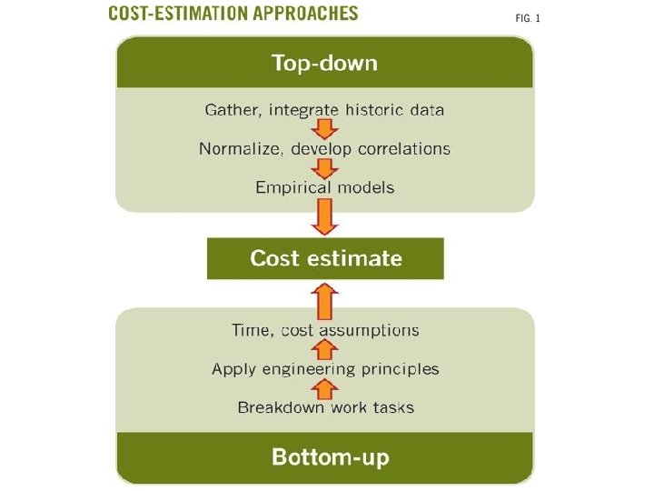
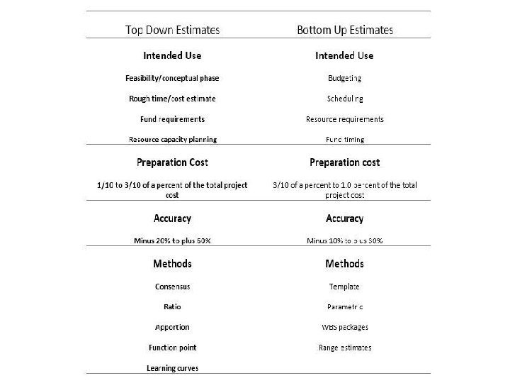
Bottom up & top down estimation • Bottom up estimation begin with lowest level parts of product or task & provide estimate for each • Combine low-level estimate into higher level one, it is applies to decomposition technique only • Top –down estimate begin with overall process or product • Full estimate is made & then estimate for component parts are calculated

MODEL OF COST & EFFORT • Cost model: • Provides direct estimate of effort or duration • Based on empirical data reflecting factors that contribute to overall project cost • It has one primary i/p & no. of secondary adjustment factors known as cost drivers • Cost drivers are characteristic of project, process, product or resource that affects the effort or duration • Constraint model: • Demonstrate relationship over time between 2 or more parameter of effort, duration or staffing level • Rayleigh curve is used as constraint model in several commercial product

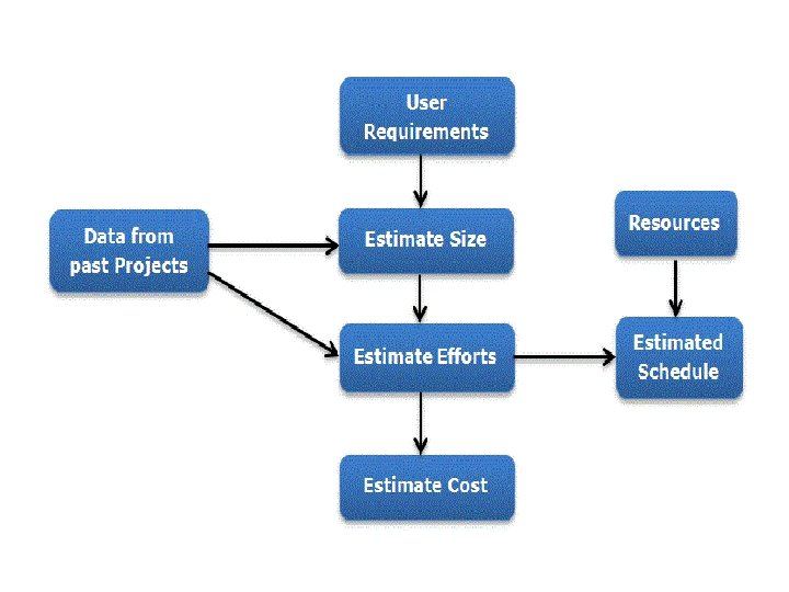
1. Regression based Model: • It is used to build cost model by collecting data from past projects & examining relationship among attributes • Once basic equation is define, estimate can be adjusted by other secondary cost factors • In fig. it indicate, how much a regression equation can be derived

• Each data point represent a project • Regression has been performed using logarithm of physical size on X-axis & log of project effort on Y-axis • Transforming linear equation: - log E = log a + b log S • Log-log domain to real domain yield an exponential relationship of form E = a Sb

• If size were a perfect predictor of effort then every point of graph would lies on line of equation with residual error zero • Next step: - identify factor that cause variation between predicted & actual effort • Factor analysis help to identify additional parameter • Add this factor to model as cost driver & assign weighting factors to model their effort • Weight are applied to R. H. S. of effort equation E=(a. Sb). F

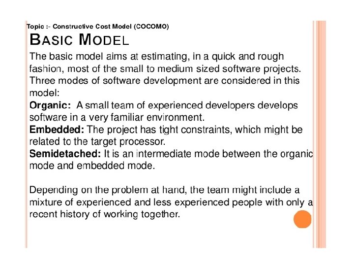
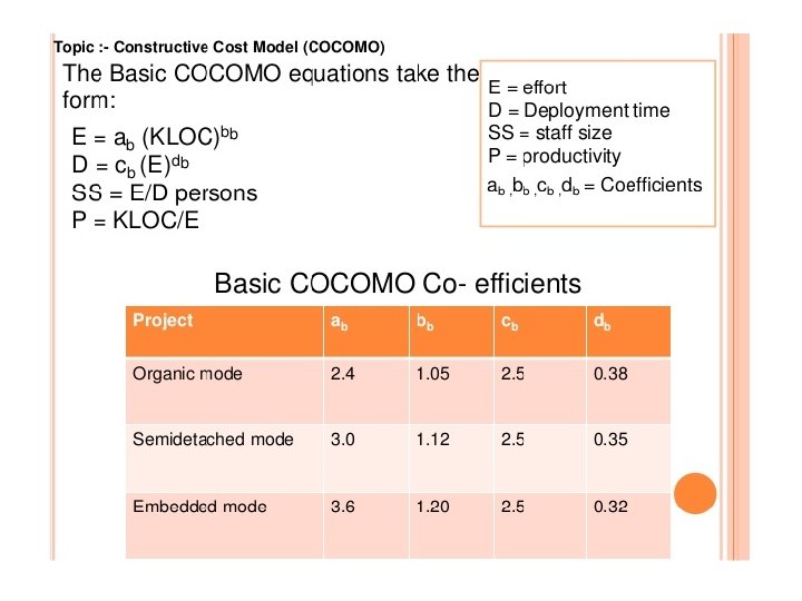
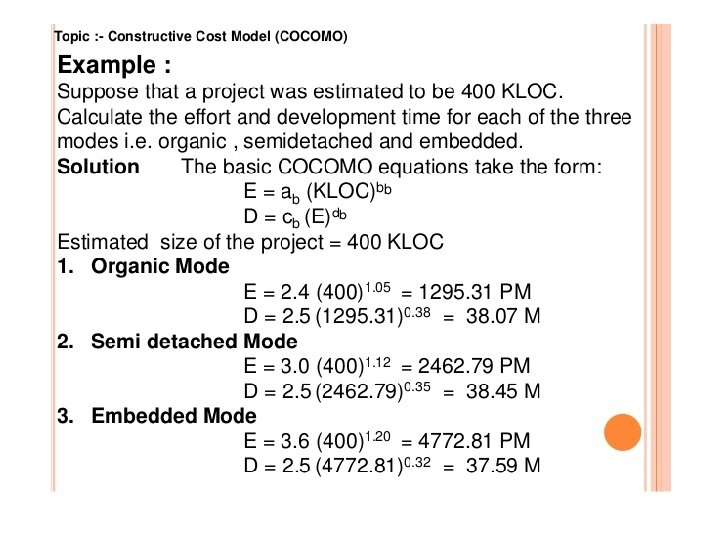
2. COCOMO: A. ORIGINAL COCOMO MODEL: -EFFORT • Collection of 3 models • • • Basic model: - applied when little about project is known Intermediate model: - applied after requirement are specified Advanced model: - applied when design is completed All 3 take same form E =a. Sb. F E= effort in person month, S= size in KDSI F = adjustment factor • Value of a & b depend on development model determined by type of s/w under construction

• Value of a & b depend on development model determined by type of s/w under construction Development mode a b organic 2. 4 1. 05 Semi-detached 3. 0 1. 12 embedded 3. 6 1. 20 Fig: - effort parameter for three modes of COCOMO • Organic system: - involve data processing - It tend to use d/b & focus on transaction & data retrieval Ex: - banking or accounting system • Embedded system: -contain real time s/w that is integral part of large h/w based system Ex: - missile guidance system • Semi-detached: - Between organic & embedded

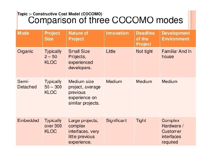
Team Size Organic Semi-Detach Embedded Small Size Medium Size Large Size 2 -50 KLOC 50 -300 KLOC 300 & Above KLOC Experienced Developers needed Average Experienced peoples Very Little previous experience Size Developers experiences Significant Environment changes (Almost new env. ) Less Familiar Environment Innovation Little Medium Major Deadline Not Tight Medium Tight E. g. Payroll System Utility System Air Traffic Control System

B. ORIGINAL COCOMO: DURATION • • Predict elapsed time from effort Same form as effort D=a Eb. F D= duration in month • Co-efficient & exponent depend on development mode, it give optimal estimate of project duration for a given effort Development mode a b organic 2. 5 0. 38 Semi-detached 2. 5 0. 35 embedded 2. 5 0. 32

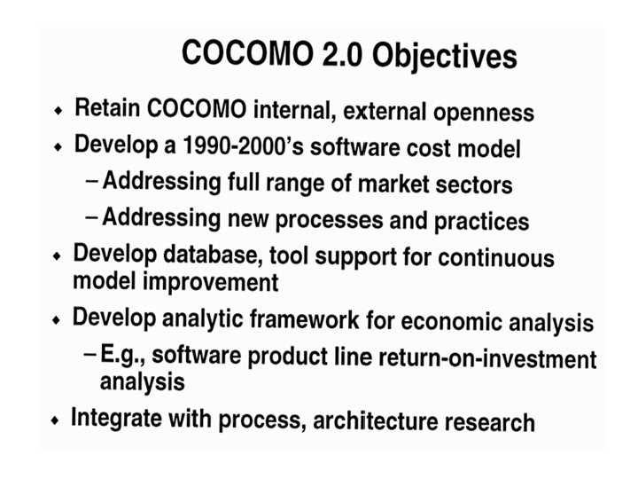
In COCOMO 2. 0 Stage 1: - - Project builds prototype to resolve high risk issues involving user interface, s/w & system interaction, performance or technological maturity - Little is known about size of final product - Estimates the size in terms of object –point Stage 2: - Designer explore alternative architecture & concept of operation - Again not enough info. To support effort & duration, but more as compare to stage 1

In COCOMO 2. 0 - Estimate the size in terms of function point, estimate functionality of product Stage 3: - - Development begun & more information is known - This stage correspond to original COCOMO model - Estimates the size in term of LOC

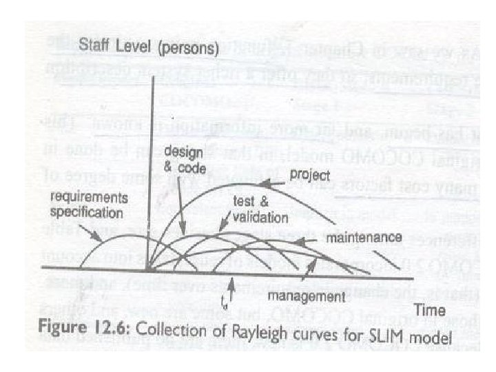
3. Putnam’s SLIM model: -Putnam develop constraint model called SLIM - Applied to project exceeding 70, 000 LOC - It assume that effort for s/w development. Project is distributed similarly to a collection of Rayleigh curves, one for each major development activity as shown in fig: -

• Putnam use empirical observations about productivity level to derive s/w equation from Rayleigh curve formula • This equation relates size to several variables: technology factor C, total project effort measured in person year K, & elapsed time to delivery td in year • Relationship expressed as – td is a point at which Rayleigh curve reaches a maximum - C takes up to 20 different values - SLIM eq. include 4 th power-strong implication for resource allocation on large project

Putnam's SLIM Model • To estimate effort/duration, Putnam introduce: • D 0 = K / td 3 • D 0 - manpower acceleration constant (12. 3 for new software with many interface and interactions with other system), 15 for stand-alone system, 27 for re-implementation of existing systems)

• To allow effort or duration estimation, Putnam derived the equation – Ex: - 12. 3 - for manpower acceleration 15 - for stand alone system 27 - for reimplementation of existing system • These values obtain from studies of existing system • By combining equation 1 & 2, Putnam derived equation for Effort as • SLIM uses separate Rayleigh curve for 1. 2. 3. 4. Design & code Test & validation Maintenance management

Multi-project models • Effort estimates are affected by other projects • Cost can be amortized over several upcoming projects. • Reuse normally involves multiple projects

S/W Documentation: ü Describe how document is checked for accuracy & also describe criteria for document distribution ü Need to get clear idea about our product & to make it user friendly ü Minimum components of documentation set include: 1. 2. 3. 4. 5. 6. 7. s/w Requirement Specification(SRS) s/w Design Description (SDD) s/w Interface Documentation (SID) s/w Test Documentation (STD) s/w Development plan(SDP) User Documentation Document Distribution

1. Software Requirement Specification(SRS) • • Describe capabilities , states & functionalities of all aspect of system Include major component & subcomponents and internal interfaces of s/w & d/b Include items required by user This type of documentation need to be prepare for each deliverable & nondeliverable item of s/w , firmware & h/w 2. Software Design Description (SDD) Describe major component & subcomponents of s/w including d/b , internal interfaces • Include use of computerized design tool • Design & coding standards are used in development of deliverable & nondeliverable item of s/w •

3. Software Interface Documentation (SID) • Describe capabilities & functionalities of all interfaces between any two component of system. • Include major component & subcomponents and both internal & external interfaces of s/w. 4. Software Test Documentation • Include 1. Test design procedure & specification 2. Test log 3. Test Summary Report

5. Software Development Plan • No good standard for it. Even ISO 9000 doesn’t require it • Whatever format choose to use , come up with format , get everyone agree on it & finalize to it • Consistency is very important in SDP 6. User Documentation • It describes the req. i/p , options & other user activities necessary for successful use & application of system • 2 - objective • To train user to get help & accurate service from system • Provide effective on-going reference for usage of system

7. Document Distribution • Process Interface to Configuration Management: ü Interface between document distribution function & s/w configuration mgmt. function need to be define for purpose of document distribution ü All procedure are needed to defined & implemented for all document before their distribution • Distribution to Internal Project Personnel ü Procedure for distribution of system document to internal project personnel must be clearly defined • Distribution to External Project Personnel ü Procedure for distribution of system document to external project personnel must be clearly defined

PROBLEM WITH EXISTING MODELING METHODS • Model accuracy evaluation take one of two form 1. Study applied model to past project data from no. of projects & compare actual effort with predicted effort 2. Study use a selection of models to estimate effort for particular project -Reason of existing modeling method fail in their goals: - 1. Model structure: ü ü Key determinant of effort is size But relation between effort & size is unclear Value of a & b differ from data set to data set most model include adjustment for diseconomy of scale

ü Putnam model implies that decreasing duration increase effort, but increasing duration decrease effort ü Most model perform poorly because they developed from post-hoc analysis of particular data set 2. Overlay complex models -many model include adjustment factors such as COCOMO cost factor & SLIM’s technology factor to provide flexibility - Cost driver doesn’t always improve accuracy of estimate 3. Product size estimation -size is not measurable early in life cycle - COCOMO & SLIM req. size in LOC but LOC can’t be measured from req. document - Estimate of LOC may be very inaccurate

DEALING WITH PROBLEMS OF CURRENT ESTIMATION METHODS -step to improve accuracy of prediction 1. Local data definitions: - Use size & effort measure that are defined consistently across the environment Measure must be understandable by all who use & 2 people measuring should produce same no. of rating 2. Calibration: - It improve accuracy of all models. Ensuring that values supplied to model are consistent with model requirement & expectations Calibration can’t regarded as one time activity Model must be re-evaluated & re-calibrated periodically

DEALING WITH PROBLEMS OF CURRENT ESTIMATION METHODS 3. Independent estimation group: -Assign estimation responsibility to a specific group of people - Group provide estimate to all project, storing result of all data capture & analysis in historical d/b • Advantages: 1. Group member are familiar with estimation & calibration technique so consistent from one project to another 2. Estimation experience gives better sense of when project deviating from average or standard so adjust factor are realistic 3. By monitoring d/b, group can identify trends & perform analysis that are impossible for single project

- Group can re-estimate periodically 4. Reduce i/p subjectivity: - gives accurate estimation model based on homogeneous data set 5. Preliminary estimate & re-estimation: - - Estimate improve by 2 –steps Basing preliminary estimate on measure of available product & reestimating as more info. Available & more product produced A. Group estimate: -derive preliminary estimate from group -individual get experienced with wide variety of project - It is done by wideband Delphi technique

Basic procedure: 1. Co-ordinator present each expert with a specification of proposed project & info. 2. Co-ordinator call a group meeting, expert ask a question & discuss estimate issue 3. Each expert provide a initial estimate of total project & develop effort, estimate provide a range between a upper & lower bound 4. Co-ordinator prepare & circulate a summary report, indicating individual & group estimate 5. Hold meeting to discuss current estimate 6. Finally expert provides anonymous estimate, repeat step 2 to 6 satisfactory until

estimate= lower bound + 4(most likely)+upper bound 6 i. e. Group estimate is average of individual estimate Variance = upper bound-lower bound 6 B. Estimation by analogy: - Effort & duration are compare with same completed project C. Re-estimation: -

6. Alternative size measure for cost estimation - Function bang: - no. of primitive in DFD Data bang : - no. of entities in ER diagram Also measure: No. of diagram - no. of processes - amount of data No. of terminal processes – no. of processes in issued document 7. Locally develop cost model: - - 5 -steps in defining local cost model a) Decompose cost model: - Identify phrases & activities then, Suggest no. of cost model require & form basic sources of data for them

b) Formulate cost theory: - Describe relation between i/p & o/p c) Collect data: - To check validity, collect data on project that is completed in particular environment represented by local model - Theoretically 3 project to test cost theory of i/p Practically 7 to 10 project d) Analyze data & evaluate model: - Regression analysis used to analyze e) Check model: - Mean magnitude of relative error , PRED(0. 25), & EQF used to determine accurate estimate

IMPLICATION FOR PROCESS PREDICTION • Want to predict how many requirement will change during development or no. of req. fault we can expect to find during inspection • Want to predict size or complexity of design from req. , amount of design that can be reuse from past project • No. of design fault • Needed to predict when coding will be complete , how much code will be reusable on future project

IMPLICATION FOR PROCESS PREDICTION • When integration & system testing can begin • When testing will complete & when product turnover to customer • Each is collection of activities with a clears starting & end point & involve uncertainty • Making accurate predicting is challenging but necessary part of software engineering