UNIT III Searching and Sorting Subject Name PMDS

UNIT III : Searching and Sorting Subject Name : PMDS Subject Code : BECME 304 T Prof. J. Rajurkar Department of Computer Engineering, MIET, Bhandara.

Searching and Sorting Topics Searching Techniques Linear Search Binary Search Sorting Techniques Bubble Sort Insertion Sort Selection Sort Merge Sort Radix Sort

Searching Techniques

Common Problems: There are some very common problems that we use computers to solve: Searching through a lot of records for a specific record or set of records Placing records in order, which we call sorting. There are numerous algorithms to perform searches and sorts. We will briefly explore a few common ones.

Linear Search Function Template linear. Search Function template linear. Search compares each element of an array with a search key. Because the array is not in any particular order, it’s just as likely that the search key will be found in the first element as the last. On average, therefore, the program must compare the search key with half of the array’s elements. To determine that a value is not in the array, the program must compare the search key to every array element. Linear search works well for small or unsorted arrays. However, for large arrays, linear searching is inefficient. If the array is sorted (e. g. , its elements are in ascending order), you can use the high-speed binary search technique.
")
Linear Search(Cont. . )
")
Linear Search(Cont. . )
")
Linear Search(Cont. . )

Binary Search: The binary search algorithm is more efficient than the linear search algorithm, but it requires that the array first be sorted. This is only worthwhile when the vector, once sorted, will be searched a great many times—or when the searching application has stringent performance requirements. The first iteration of this algorithm tests the middle array element. If this matches the search key, the algorithm ends.
 Assuming the array is sorted in ascending order, then if")
Binary Search (cont. ) Assuming the array is sorted in ascending order, then if the search key is less than the middle element, the search key cannot match any element in the array’s second half so the algorithm continues with only the first half (i. e. , the first element up to, but not including, the middle element). If the search key is greater than the middle element, the search key cannot match any element in the array’s first half so the algorithm continues with only the second half (i. e. , the element after the middle element through the last element). Each iteration tests the middle value of the array’s remaining elements. If the element does not match the search key, the algorithm eliminates half of the remaining elements. The algorithm ends either by finding an element that matches the search key or by reducing the sub-array to zero size.
 Binary Search Example Figure 20. 3 implements and demonstrates the")
Binary Search (cont. ) Binary Search Example Figure 20. 3 implements and demonstrates the binary-search algorithm. Throughout the program’s execution, we use function template display. Elements (lines 11– 22) to display the portion of the array that’s currently being searched.
")
Binary Search (cont. )
")
Binary Search (cont. )
")
Binary Search (cont. )
")
Binary Search (cont. )
")
Binary Search (cont. )
")
Binary Search (cont. )
")
Binary Search (cont. )

Sorting Algorithms

ØSorting data (i. e. , placing the data into some particular order, such as ascending or descending) is one of the most important computing applications. ØYour algorithm choice affects only the algorithm’s runtime and memory use. ØThe next two sections introduce the selection sort and insertion sort— simple algorithms to implement, but not efficient. ØIn each case, we examine the efficiency of the algorithms using Big O notation. ØWe then present the merge sort algorithm, which is much faster but is more difficult to implement.

Insertion Sort Figure 20. 4 uses insertion sort—a simple, but inefficient, sorting algorithm—to sort a 10 -element array’s values into ascending order. Function template insertion. Sort (lines 9– 28) implements the algorithm.
")
Insertion Sort (Cont. . )
")
Insertion Sort (Cont. . )
 Insertion Sort Algorithm The algorithm’s first iteration takes the")
Insertion Sort (Cont. . ) Insertion Sort Algorithm The algorithm’s first iteration takes the array’s second element and, if it’s less than the first element, swaps it with the first element (i. e. , the algorithm inserts the second element in front of the first element). The second iteration looks at the third element and inserts it into the correct position with respect to the first two elements, so all three elements are in order. At the ith iteration of this algorithm, the first i elements in the original array will be sorted.
 First Iteration Lines 33– 34 declare and initialize the")
Insertion Sort (Cont. . ) First Iteration Lines 33– 34 declare and initialize the array named data with the following values: 34 56 4 10 77 51 93 30 5 52 Line 42 passes the array to the insertion. Sort function, which receives the array in parameter items. The function first looks at items[0] and items[1], whose values are 34 and 56, respectively. These two elements are already in order, so the algorithm continues—if they were out of order, the algorithm would swap them.
 Second Iteration In the second iteration, the algorithm looks")
Insertion Sort (Cont. . ) Second Iteration In the second iteration, the algorithm looks at the value of items[2] (that is, 4). This value is less than 56, so the algorithm stores 4 in a temporary variable and moves 56 one element to the right. The algorithm then determines that 4 is less than 34, so it moves 34 one element to the right. At this point, the algorithm has reached the beginning of the array, so it places 4 in items[0]. The array now is 4 34 56 10 77 51 93 30 5 52
 Third Iteration and Beyond In the third iteration, the")
Insertion Sort (Cont. . ) Third Iteration and Beyond In the third iteration, the algorithm places the value of items[3] (that is, 10) in the correct location with respect to the first four array elements. The algorithm compares 10 to 56 and moves 56 one element to the right because it’s larger than 10. Next, the algorithm compares 10 to 34, moving 34 right one element. When the algorithm compares 10 to 4, it observes that 10 is larger than 4 and places 10 in items[1]. The array now is 4 10 34 56 77 51 93 30 5 52 Using this algorithm, after the ith iteration, the first i + 1 array elements are sorted. They may not be in their final locations, however, because the algorithm might encounter smaller values later in the array.
 Function Template insertion. Sort Function template insertion. Sort performs")
Insertion Sort (Cont. . ) Function Template insertion. Sort Function template insertion. Sort performs the sorting in lines 13– 27, which iterates over the array’s elements. In each iteration, line 15 temporarily stores in variable insert the value of the element that will be inserted into the array’s sorted portion. Line 16 declares and initializes the variable move. Index, which keeps track of where to insert the element. Lines 19– 24 loop to locate the correct position where the element should be inserted. The loop terminates either when the program reaches the array’s first element or when it reaches an element that’s less than the value to insert. Line 22 moves an element to the right, and line 23 decrements the position at which to insert the next element. After the while loop ends, line 26 inserts the element into place. When the for statement in lines 13– 27 terminates, the array’s elements are sorted.

Selection Sort Figure 20. 5 uses the selection sort algorithm—another easy-toimplement, but inefficient, sorting algorithm—to sort a 10 -element array’s values into ascending order. Function template selection. Sort (lines 9– 27) implements the algorithm.
")
Selection Sort (Cont. . )
")
Selection Sort (Cont. . )
 Selection Sort Algorithm The algorithm’s first iteration of the")
Selection Sort (Cont. . ) Selection Sort Algorithm The algorithm’s first iteration of the algorithm selects the smallest element value and swaps it with the first element’s value. The second iteration selects the second-smallest element value (which is the smallest of the remaining elements) and swaps it with the second element’s value. The algorithm continues until the last iteration selects the second-largest element and swaps it with the second-to-last element’s value, leaving the largest value in the last element. After the ith iteration, the smallest i values will be sorted into increasing order in the first array elements.
 First Iteration Lines 32– 33 declare and initialize the")
Selection Sort (Cont. . ) First Iteration Lines 32– 33 declare and initialize the array named data with the following values: 34 56 4 10 77 51 93 30 5 52 The selection sort first determines the smallest value (4) in the array, which is in element 2. The algorithm swaps 4 with the value in element 0 (34), resulting in 4 56 34 10 77 51 93 30 5 52 Second Iteration The algorithm then determines the smallest value of the remaining elements (all elements except 4), which is 5, contained in element 8. The program swaps the 5 with the 56 in element 1, resulting in 4 5 34 10 77 51 93 30 56 52
 Third Iteration On the third iteration, the program determines")
Selection Sort (Cont. . ) Third Iteration On the third iteration, the program determines the next smallest value, 10, and swaps it with the value in element 2 (34). 4 5 10 34 77 51 93 30 56 52 The process continues until the array is fully sorted. 4 5 10 30 34 51 52 56 77 93 After the first iteration, the smallest element is in the first position; after the second iteration, the two smallest elements are in order in the first two positions and so on. Function Template selection. Sort Function template selection. Sort performs the sorting in lines 13– 26.
 Merge sort is an efficient sorting algorithm but is")
Merge Sort (A Recursive Implementation) Merge sort is an efficient sorting algorithm but is conceptually more complex than insertion sort and selection sort. The merge sort algorithm sorts an array by splitting it into two equalsized sub-arrays, sorting each sub-array then merging them into one larger array. Merge sort performs the merge by looking at each sub-arrays first element, which is also the smallest element in that sub-array. Merge sort takes the smallest of these and places it in the first element of merged, sorted array. If there are still elements in the sub-arrays, merge sort looks at the second element in that sub-array (which is now the smallest element remaining) and compares it to the first element in the other sub-array.
 (cont. . ) Merge sort continues this process until")
Merge Sort (A Recursive Implementation) (cont. . ) Merge sort continues this process until the merged array is filled. Once a sub-array has no more elements, the merge copies the other array’s remaining elements into the merged array.
 (cont. . ) Demonstrating Merge Sort Figure 20. 6")
Merge Sort (A Recursive Implementation) (cont. . ) Demonstrating Merge Sort Figure 20. 6 implements and demonstrates the merge sort algorithm. Throughout the program’s execution, we use function template display. Elements (lines 10– 21) to display the portions of the array that are currently being split and merged. Function templates merge. Sort (lines 24– 49) and merge (lines 52– 98) implement the merge sort algorithm. Function main (lines 100– 125) creates an array, populates it with random integers, executes the algorithm (line 120) and displays the sorted array. The output from this program displays the splits and merges performed by merge sort, showing the progress of the sort at each step of the algorithm.
 (cont. . )")
Merge Sort (A Recursive Implementation) (cont. . )
 (cont. . )")
Merge Sort (A Recursive Implementation) (cont. . )
 (cont. . )")
Merge Sort (A Recursive Implementation) (cont. . )
 (cont. . )")
Merge Sort (A Recursive Implementation) (cont. . )
 (cont. . )")
Merge Sort (A Recursive Implementation) (cont. . )
 (cont. . )")
Merge Sort (A Recursive Implementation) (cont. . )
 (cont. . )")
Merge Sort (A Recursive Implementation) (cont. . )
 (cont. . )")
Merge Sort (A Recursive Implementation) (cont. . )
 (cont. . )")
Merge Sort (A Recursive Implementation) (cont. . )
 (cont. . )")
Merge Sort (A Recursive Implementation) (cont. . )
 (cont. . ) Function merge. Sort Recursive function merge.")
Merge Sort (A Recursive Implementation) (cont. . ) Function merge. Sort Recursive function merge. Sort (lines 24– 49) receives as parameters the array to sort and the low and high indices of the range of elements to sort. Line 28 tests the base case. If the high index minus the low index is 0 (i. e. , a one-element subarray), the function simply returns. If the difference between the indices is greater than or equal to 1, the function splits the array in two—lines 30– 31 determine the split point.
 (cont. . ) Next, line 43 recursively calls function")
Merge Sort (A Recursive Implementation) (cont. . ) Next, line 43 recursively calls function merge. Sort on the array’s first half, and line 44 recursively calls function merge. Sort on the array’s second half. When these two function calls return, each half is sorted. Line 47 calls function merge (lines 52– 98) on the two halves to combine the two sorted arrays into one larger sorted array.
 (cont. . )")
Merge Sort (A Recursive Implementation) (cont. . )
 (cont. . )")
Merge Sort (A Recursive Implementation) (cont. . )
 (cont. . )")
Merge Sort (A Recursive Implementation) (cont. . )
 (cont. . )")
Merge Sort (A Recursive Implementation) (cont. . )
 (cont. . )")
Merge Sort (A Recursive Implementation) (cont. . )
 (cont. . )")
Merge Sort (A Recursive Implementation) (cont. . )
 (cont. . ) Function merge Lines 69– 77 in")
Merge Sort (A Recursive Implementation) (cont. . ) Function merge Lines 69– 77 in function merge loop until the program reaches the end of either sub-array. Line 73 tests which element at the beginning of the two sub-arrays is smaller. If the element in the left sub-array is smaller or both are equal, line 74 places it in position in the combined array. If the element in the right sub-array is smaller, line 76 places it in position in the combined array. When the while loop completes, one entire sub-array is in the combined array, but the other sub-array still contains data. Line 79 tests whether the left sub-array has reached the end. If so, lines 81– 82 fill the combined array with the elements of the right sub-array.
 (cont. . ) If the left sub-array has not")
Merge Sort (A Recursive Implementation) (cont. . ) If the left sub-array has not reached the end, then the right subarray must have reached the end, and lines 86– 87 fill the combined array with the elements of the left sub-array. Finally, lines 91– 92 copy the combined array into the original array.
![Bubble Sort void bubble. Sort (int a[ ] , int size) { int i,](http://slidetodoc.com/presentation_image_h2/2e9ca1d79d2ed4f7556a0dd2aa6df455/image-58.jpg "Bubble Sort void bubble. Sort (int a[ ] , int size) { int i,")
Bubble Sort void bubble. Sort (int a[ ] , int size) { int i, j, temp; for ( i = 0; i < size; i++ ) /* controls passes through the list */ { for ( j = 0; j < size - 1; j++ ) /* performs adjacent comparisons */ { if ( a[ j ] > a[ j+1 ] ) /* determines if a swap should occur */ { temp = a[ j ]; /* swap is performed */ a[ j ] = a[ j + 1 ]; a[ j+1 ] = temp; } }

Radix Sort If your integers are in a larger range then do bucket sort on each digit Start by sorting with the low-order digit using a STABLE bucket sort. Then, do the next-lowest, and so on.
")
Radix Sort (Cont. . )
 Radix sort can be used for decimal numbers and")
Radix Sort (Cont. . ) Radix sort can be used for decimal numbers and alphanumeric strings.

What is mean by Hashing? Explain different Collision resolution policies. Hashing is the process of mapping large amount of data item to a smaller table with the help of a hashing function. The essence of hashing is to facilitate the next level searching method when compared with the linear or binary search. The advantage of this searching method is its efficiency to hand vast amount of data items in a given collection (i. e. collection size). Due to this hashing process, the result is a Hash data structure that can store or retrieve data items in an average time disregard to the collection size. Hash Table is the result of storing the hash data structure in a smaller table which incorporates the hash function within itself. The Hash Function primarily is responsible to map between the original data item and the smaller table itself.

Characteristics of a Good Hash Function ØThe hash value is fully determined by the data being hashed. ØThe hash function uses all the input data. ØThe hash function "uniformly" distributes the data across the entire set of possible hash values. ØThe hash function generates very different hash values for similar strings. Types of hashing Division Hash Method The Folding Method The Mid- Square Method

Division Hash Method The key K is divided by some number m and the remainder is used as the hash address of K. h(k)=k mod m This gives the indexes in the range 0 to m-1 so the hash table should be of size m. This is an example of uniform hash function if value of m will be chosen carefully. Generally a prime number is a best choice which evenly. will spread keys A uniform hash function is designed to distribute the keys roughly evenly into the available positions within the array (or hash table).

The Folding Method The key K is partitioned into a number of parts each of which has the same length as the required address with the possible exception of the last part. The parts are then added together ignoring the final carry, to form an address. Example: If key=356942781 is to be transformed into a three digit address. P 1=356, P 2=942, P 3=781 are added to yield 079. (i. e 356+942+781=2079 , ignoring carry 2 )

The Mid- Square Method The key K is multiplied by itself and the address is obtained by selecting an appropriate number of digits from the middle of the square. The number of digits selected depends on the size of the table. Example: If key=123456 is to be transformed. (123456)2=15241383936 If a three-digit address is required, positions 5 to 7 could be chosen giving address 138. Hashing has time complexity O (1) and is quite fast in practice.

Collision Resolution When two or more entries may comes on same hash value, then concept of collision resolution applies. There are fallowing strategies to solve collision Separate chaining Open addressing Linear probing Quadratic probing Double hashing

Separate Chaining The last strategy we discuss is the idea of separate chaining. The idea here is to resolve a collision by creating a linked list of elements as shown below.
 In the picture above the objects, “As”, “foo”, and “bar”")
Separate Chaining(Cont. . ) In the picture above the objects, “As”, “foo”, and “bar” all hash to the same location in the table, that is A[0]. So we create a list of all the elements that hash into that location. Similarly, all other lists indicate keys that were hashed into the same location.

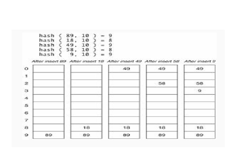
Linear Probing Suppose that a key hashes into a position that is already occupied. The simplest strategy is to look for the next available position to place the item. Suppose we have a set of hash codes consisting of {89, 18, 49, 58, 9} and we need to place them into a table of size 10. The following table demonstrates this process. Algorithm Linear. Probing. Insert(k) If (table is full) error Probe = h(k) While( table [probe] occupied) Probe = (probe+1) mod m Table[probe] = k
")
Linear Probing (Contd. )
 The first collision occurs when 49 hashes to the same")
Linear Probing (Contd. ) The first collision occurs when 49 hashes to the same location with index 9. Since 89 occupies the A[9], we need to place 49 to the next available position. Considering the array as circular, the next available position is 0. That is (9+1) mod 10. So we place 49 in A[0]. Several more collisions occur in this simple example and in each case we keep looking to find the next available location in the array to place the element. Now if we need to find the element, say for example, 49, we first compute the hash code (9), and look in A[9]. Since we do not find it there, we look in A[(9+1) % 10] = A[0], we find it there and we are done. So what if we are looking for 79? First we compute hashcode of 79 = 9. We probe in A[9], A[(9+1)%10]=A[0], A[(9+2)%10]=A[1], A[(9+3)%10]=A[2], A[(9+4)%10]=A[3] etc. Since A[3] = null, we do know that 79 could not exists in the set.

Quadratic Probing Although linear probing is a simple process where it is easy to compute the next available location, linear probing also leads to some clustering when keys are computed to closer values. Therefore we define a new process of Quadratic probing that provides a better distribution of keys when collisions occur. In quadratic probing, if the hash value is K , then the next location is computed using the sequence K + 1, K + 4, K + 9 etc. . Formula hi (k) = (hash(k) + i 2) mod size The following table shows the collision resolution using quadratic probing.
")
Double Hashing It uses two hash functions h 1, h 2. h 1 (K) is the position in the table where we first check for key k. h 2 (K) determines that offset we use when searching for k. In linear probing h 2 (K) is always 1. Algorithm Double. Hashing. Insert(k) If (table is full) error Probe = h 1(k) offset =h 2(k) While( table [probe] occupied) Probe = (probe+offset) mod m Table [probe] = k
 If after adding offset is space is not vacant,")
Double Hashing (Cont. . ) If after adding offset is space is not vacant, then add offset again for searching next space. Example: H 1(K) = k mod 13 H 2(K) = 8 - (k mod 8) Insert keys = 18, 41, 22, 44, 59, 32, 31, 73
- Slides: 76