Unit II Image Enhancement and Restoration Spatial domain

Unit II: Image Enhancement and Restoration Spatial domain enhancement: Point operations-Log transformation, Power-law transformation, Piecewise linear transformations, Histogram equalization. Filtering operations- Image smoothing, Image sharpening. Frequency domain enhancement: 2 D DFT, Smoothing and Sharpening in frequency domain. Homomorphic filtering. Restoration: Noise models, Restoration using Inverse filtering and Wiener filtering

Enhancement Techniques Spatial Operates on pixels Frequency Domain Operates on FT of Image

What Is Image Enhancement? Image enhancement is the process of making images more useful In this technique image is processed so that the resultant image is more suitable than the original for specific applications i. e image is enhanced. The reasons for doing this include: – Highlighting interesting detail in images – Removing noise from images – Making images more visually appealing

Images taken from Gonzalez & Woods, Digital Image Processing (2002) Image Enhancement Examples

Images taken from Gonzalez & Woods, Digital Image Processing (2002) Image Enhancement Examples (cont…)

Images taken from Gonzalez & Woods, Digital Image Processing (2002) Image Enhancement Examples (cont…)

Spatial & Frequency Domains There are two broad categories of image enhancement techniques – Spatial domain techniques • Direct manipulation of image pixels – Frequency domain techniques • Manipulation of Fourier transform or wavelet transform of an image For the moment we will concentrate on techniques that operate in the spatial domain

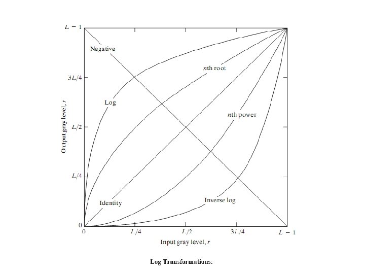
Special domain methods includes: - point processing and Neighbourhood processing(Directly worked with the pixel values to get a new image). Point processing is of two types 1) Gray level transformation/point operation: Image negative/Digital negative, Log transformations, Power law transformation. 2) Piecewise linear transformation. Contrast Streching Thresholding Bit plane Slicing(Bit Extraction) Gray level slicing(Intensity Slicing) Range Compression.

Digital Negative L 0 EE 465: Introduction to Digital Image Processing L x 9

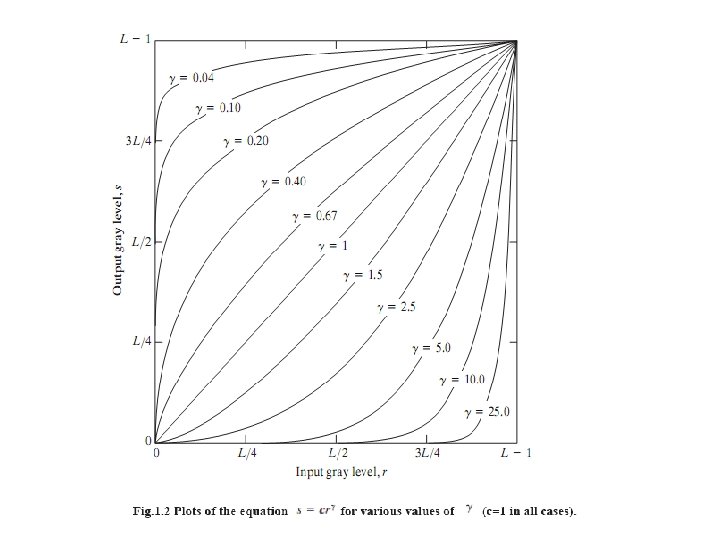
The proces used to correct this power-law response phenomena is called gamma correction. For example, cathode ray tube (CRT) devices have an intensity-to-voltage response that is a power function, with exponents varying from approximately 1. 8 to 2. 5. With reference to the curve for g=2. 5 in Fig. 1. 2, we see that such display systems would tend to produce images that are darker than All we need to do is preprocess the input before inputting It into the monitoring by performing gamma correction. This gamma corrected input produces an output that is close to original input. gamma correction is imp if displaying an image accuratelyb on a computer screen. images that are not gamma corrected properly can look either bleached out or too dark.

Piecewise-Linear Transformation Functions: The principal advantage of piecewise linear functions over the types of functions we have discussed above is that the form of piecewise functions can be arbitrarily complex.

Contrast Stretching • To increase the dynamic range of the gray levels in the image being processed.

contd… • The locations of (r 1, s 1) and (r 2, s 2) control the shape of the transformation function. – If r 1= s 1 and r 2= s 2 the transformation is a linear function and produces no changes. – If r 1=r 2, s 1=0 and s 2=L-1, the transformation becomes a thresholding function that creates a binary image. – Intermediate values of (r 1, s 1) and (r 2, s 2) produce various degrees of spread in the gray levels of the output image, thus affecting its contrast. – Generally, r 1≤r 2 and s 1≤s 2 is assumed.

Example

Contrast Stretching yb ya 0 a b L x 17

Gray-level slicing:

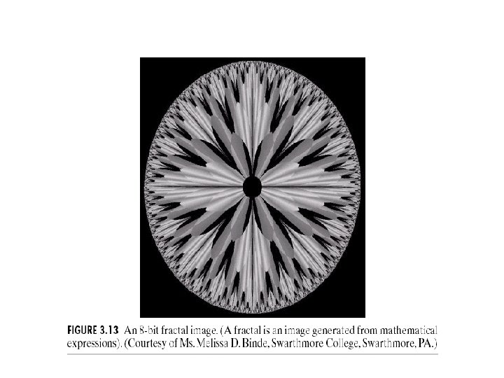
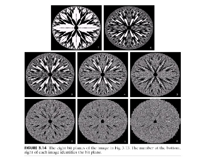
Bit-Plane Slicing • To highlight the contribution made to the total image appearance by specific bits. – i. e. Assuming that each pixel is represented by 8 bits, the image is composed of 8 1 -bit planes. – Plane 0 contains the least significant bit and plane 7 contains the most significant bit. – Only the higher order bits (top four) contain visually significant data. The other bit planes contribute the more subtle details.

Image Histograms Frequencies The histogram of an image shows us the distribution of grey levels in the image Massively useful in image processing, especially in segmentation Grey Levels

Images taken from Gonzalez & Woods, Digital Image Processing (2002) Histogram Examples (cont…)

Images taken from Gonzalez & Woods, Digital Image Processing (2002) Histogram Examples (cont…)

Images taken from Gonzalez & Woods, Digital Image Processing (2002) Histogram Examples (cont…)

Histogram Examples (cont…)

Images taken from Gonzalez & Woods, Digital Image Processing (2002) Histogram Examples (cont…)

Histogram Examples (cont…) A selection of images and their histograms Notice the relationships between the images and their histograms Note that the high contrast image has the most evenly spaced histogram x-axis – values of intensities y-axis – their frequencies

Spreading out the frequencies in an image (or equalising the image) is a simple way to improve dark or washed out images. Histogram Equalization · What is the histogram equalization? · The histogram equalization is an approach to enhance a given image. The approach is to design a transformation T(. ) such that the gray values in the output is uniformly distributed in [0, 1]. · In terms of histograms, the output image will have all gray values in “equal proportion”.

How to implement histogram equalization? Step 1: For images with discrete gray values, compute: L: Total number of gray levels nk: Number of pixels with gray value rk n: Total number of pixels in the image Step 2: Based on CDF, compute the discrete version of the previous transformation :

Example: · Consider an 8 -level 64 x 64 image with gray values (0, 1, …, 7). The normalized gray values are (0, 1/7, 2/7, …, 1). The normalized histogram is given below: NB: The gray values in output are also (0, 1/7, 2/7, …, 1).

# pixels Fraction of # pixels Gray value Normalized gray value

· Applying the transformation, we have

· Notice that there are only five distinct gray levels --- (1/7, 3/7, 5/7, 6/7, 1) in the output image. We will relabel them as (s 0, s 1, …, s 4 ). · With this transformation, the output image will have histogram

Histogram of output image # pixels Gray values · Note that the histogram of output image is only approximately, and not exactly, uniform. This should not be surprising, since there is no result that claims uniformity in the discrete case.

Example Original image and its histogram

Histogram equalized image and its histogram