UNIT II Greedy and Dynamic Programming Algorithmic Strategies

UNIT- II Greedy and Dynamic Programming Algorithmic Strategies Greedy strategy: Principle, control abstraction, time analysis of control abstraction, knapsack problem, scheduling algorithms-Job scheduling and activity selection problem. Dynamic Programming: Principle, control abstraction, time analysis of control abstraction, binomial coefficients, OBST, 0/1 knapsack, Chain Matrix multiplication.

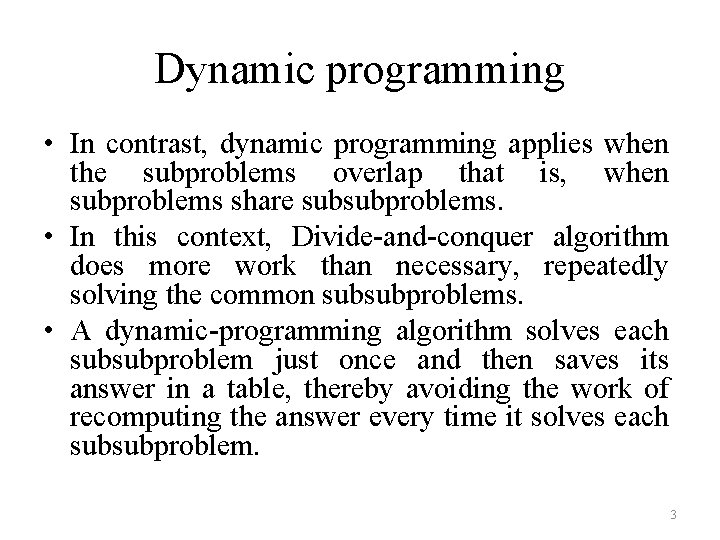
Dynamic Programming • Dynamic programming, like the divide-andconquer method, solves problems by combining the solutions to subproblems. • “Programming” in this context refers to a tabular method, not to writing computer code. • Divide-and-conquer algorithm – partition the problem into disjoint subprob-lems, – solve the subproblems recursively, – combine their solutions to solve the original problem. 2

Dynamic programming • In contrast, dynamic programming applies when the subproblems overlap that is, when subproblems share subsubproblems. • In this context, Divide-and-conquer algorithm does more work than necessary, repeatedly solving the common subsubproblems. • A dynamic-programming algorithm solves each subsubproblem just once and then saves its answer in a table, thereby avoiding the work of recomputing the answer every time it solves each subsubproblem. 3

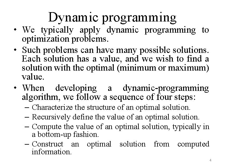
Dynamic programming • We typically apply dynamic programming to optimization problems. • Such problems can have many possible solutions. Each solution has a value, and we wish to find a solution with the optimal (minimum or maximum) value. • When developing a dynamic-programming algorithm, we follow a sequence of four steps: – Characterize the structure of an optimal solution. – Recursively define the value of an optimal solution. – Compute the value of an optimal solution, typically in a bottom-up fashion. – Construct an optimal solution from computed information. 4

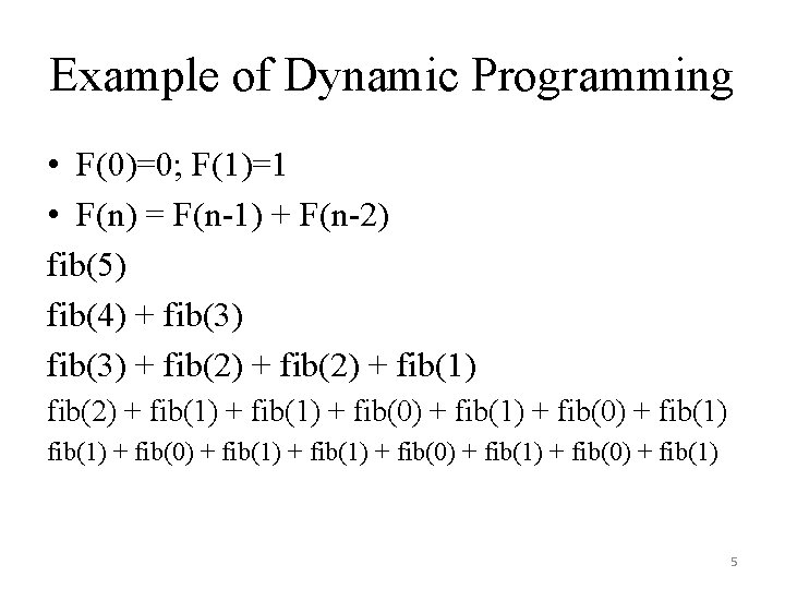
Example of Dynamic Programming • F(0)=0; F(1)=1 • F(n) = F(n-1) + F(n-2) fib(5) fib(4) + fib(3) + fib(2) + fib(1) + fib(0) + fib(1) + fib(0) + fib(1) 5

Application of Dynamic programming • • 0/1 knapsack Binomial coefficients Optimal binary search tree Matrix chain multiplication. 6

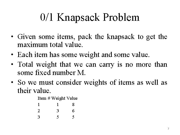
0/1 Knapsack Problem • Given some items, pack the knapsack to get the maximum total value. • Each item has some weight and some value. • Total weight that we can carry is no more than some fixed number M. • So we must consider weights of items as well as their value. Item # Weight Value 1 1 8 2 3 6 3 5 5 7

0/1 Knapsack Problem • There are two versions of the problem: • Fractional knapsack problem – Items are divisible: you can take any fraction of an item. – Solved with a greedy algorithm. • 0 -1 knapsack problem – Items are indivisible; you either take an item or not. – Solved with dynamic programming 8

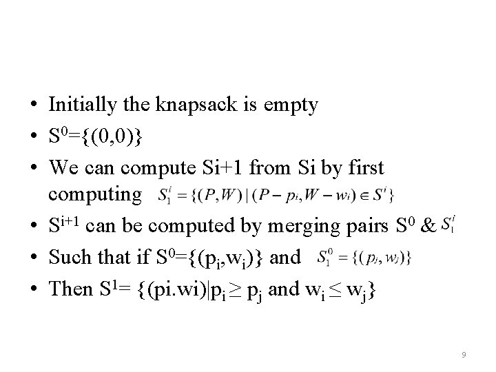
• Initially the knapsack is empty • S 0={(0, 0)} • We can compute Si+1 from Si by first computing • Si+1 can be computed by merging pairs S 0 & • Such that if S 0={(pi, wi)} and • Then S 1= {(pi. wi)|pi ≥ pj and wi ≤ wj} 9

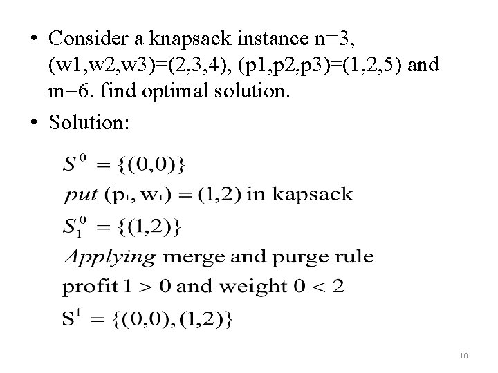
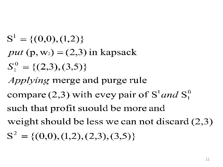
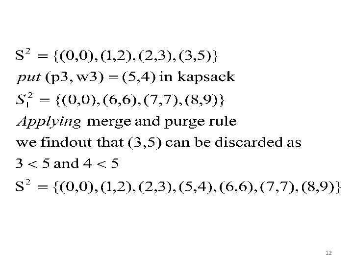
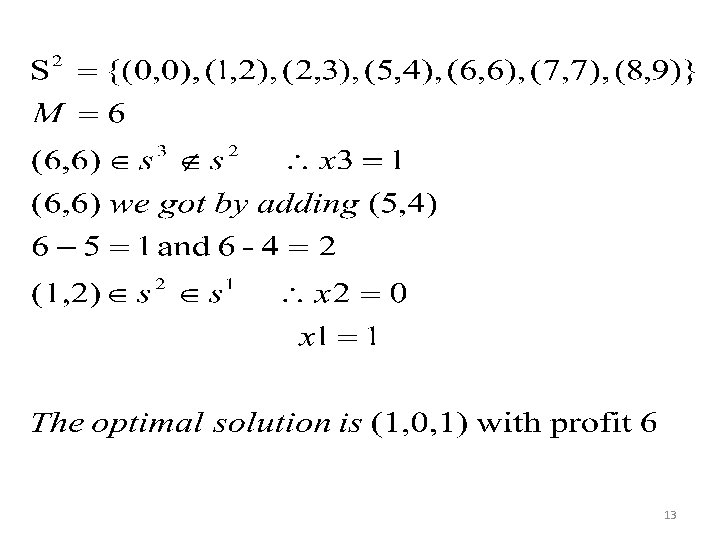
• Consider a knapsack instance n=3, (w 1, w 2, w 3)=(2, 3, 4), (p 1, p 2, p 3)=(1, 2, 5) and m=6. find optimal solution. • Solution: 10

11

12

13

14

Chain Matrix Multiplication • Matrix: An n × m matrix A=[a(i, j)] is a two dimensional array which has n rows and m columns. • The product C=AB of a p × q matrix A and a q × r matrix B is a p × r matrix given by for i ≤ p and i ≤ j ≤ r 15

Chain Matrix Multiplication • Matrix multiplication is not commutative i. e AB≠BA • Matrix multiplication is associative • A 1 A 2 A 3=(A 1 A 2)A 3=A 1(A 2 A 3) • so parenthenization does not change result. 16

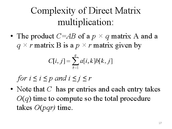
Complexity of Direct Matrix multiplication: • The product C=AB of a p × q matrix A and a q × r matrix B is a p × r matrix given by for i ≤ p and i ≤ j ≤ r • Note that C has pr entries and each entry takes O(q) time to compute so the total procedure takes O(pqr) time. 17

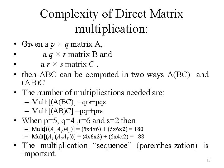
Complexity of Direct Matrix multiplication: • Given a p × q matrix A, • a q × r matrix B and • a r × s matrix C , • then ABC can be computed in two ways A(BC) and (AB)C • The number of multiplications needed are: – Multi[(A(BC)] =qrs+pqs – Multi[(AB)C] =pqr+prs • When p=5, q=4 , r=6 and s=2 then – Mult[((A 1 A 2)A 3)] = (5 x 4 x 6) + (5 x 6 x 2) = 180 – Mult[(A 1 (A 2 A 3 ))] = (4 x 6 x 2) + (5 x 4 x 2) = 88 • The multiplication “sequence” (parenthesization) is important. 18

Complexity of Direct Matrix multiplication: • When p=5, q=4 , r=6 and s=2 then – Mult[((A 1 A 2)A 3)] = (5 x 4 x 6) + (5 x 6 x 2) = 180 – Mult[(A 1 (A 2 A 3 ))] = (4 x 6 x 2) + (5 x 4 x 2) = 88 • The multiplication “sequence” (parenthesization) is important. 19

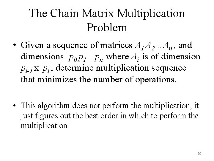
The Chain Matrix Multiplication Problem • Given a sequence of matrices A 1 A 2…An , and dimensions p 0 p 1…pn where Ai is of dimension pi-1 x pi , determine multiplication sequence that minimizes the number of operations. • This algorithm does not perform the multiplication, it just figures out the best order in which to perform the multiplication 20

Developing a Dynamic Programming Algorithm • Step 1: Determine the structure of an optimal solution (in this case, a parenthesization). • For any optimal multiplication sequence, at the last step you are multiplying two matrices Ai. . k and Ak+1. . j for some k • That is, • Ai. . j=(Ai…. Ak)(Ak+1…Aj) • A 3. . 6=A 3. . 5 A 6. . 6 21

Developing a Dynamic Programming Algorithm • Step 2: Recursively define the value of an optimal solution. • For for 1 ≤ i ≤ j ≤ n, let m[i, j] denote the minimum number of multiplications needed to compute Ai. . j. The optimum cost can be described by the following recursive definition m[i, i] = 0 m[i, j] = mini k < j (m[i, k] + m[k+1, j] + pi-1 pkpj ) for i < j 22

Computing m[i, j] • For a specific k, (Ai …Ak)( Ak+1 … Aj) = m[i, j] = mini k < j (m[i, k] + m[k+1, j] + pi-1 pkpj )

Computing m[i, j] • For a specific k, (Ai …Ak)( Ak+1 … Aj) = Ai…k( Ak+1 … Aj) (m[i, k] mults) m[i, j] = mini k < j (m[i, k] + m[k+1, j] + pi-1 pkpj )

Computing m[i, j] • For a specific k, (Ai …Ak)( Ak+1 … Aj) = Ai…k Ak+1…j (m[i, k] mults) (m[k+1, j] mults) m[i, j] = mini k < j (m[i, k] + m[k+1, j] + pi-1 pkpj )

Computing m[i, j] • For a specific k, (Ai …Ak)( Ak+1 … Aj) = Ai…k Ak+1…j = Ai…j (m[i, k] mults) (m[k+1, j] mults) (pi-1 pk pj mults) m[i, j] = mini k < j (m[i, k] + m[k+1, j] + pi-1 pkpj )

Computing m[i, j] • For a specific k, (Ai …Ak)( Ak+1 … Aj) = Ai…k Ak+1…j = Ai…j (m[i, k] mults) (m[k+1, j] mults) (pi-1 pk pj mults) • For solution, evaluate for all k and take minimum. m[i, j] = mini k < j (m[i, k] + m[k+1, j] + pi-1 pkpj )

Matrix-Chain-Order(p) 1. n length[p] - 1 2. for i 1 to n // initialization: O(n) time 3. do m[i, i] 0 4. for L 2 to n // L = length of sub-chain 5. do for i 1 to n - L+1 6. do j i + L - 1 7. m[i, j] 8. for k i to j - 1 9. do q m[i, k] + m[k+1, j] + pi-1 pk pj 10. if q < m[i, j] 11. then m[i, j] q 12. s[i, j] k 13. return m and s

Analysis • The array s[i, j] is used to extract the actual sequence (see next). • There are 3 nested loops and each can iterate at most n times, so the total running time is (n 3).

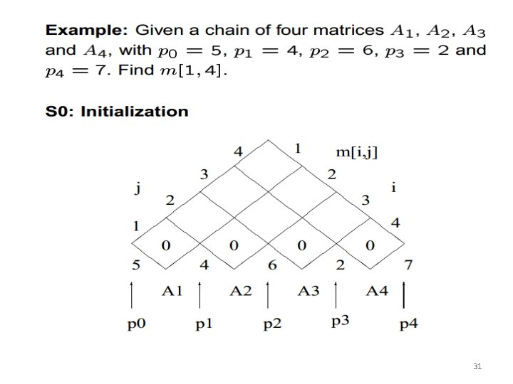
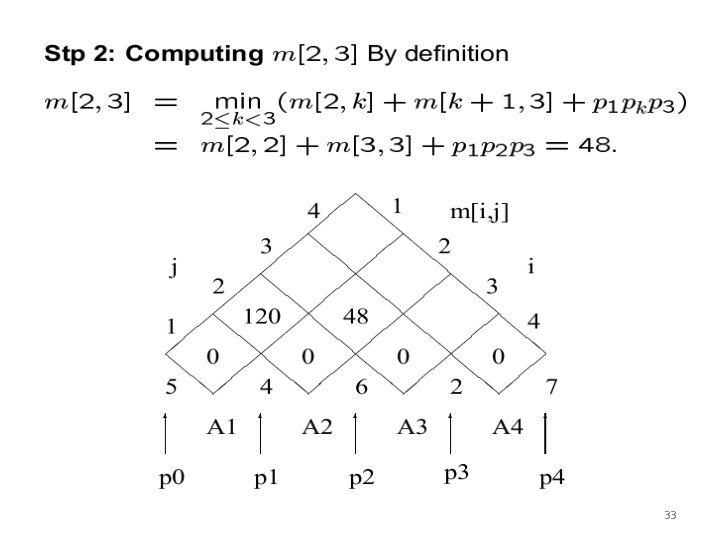
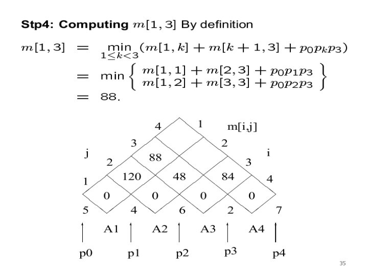
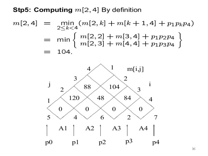
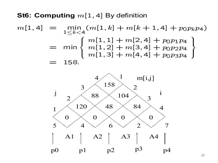
• Step 3: Compute the value of an optimal solution in a bottom-up fashion 30

31

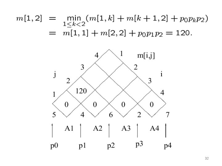
32

33

34

35

36

37

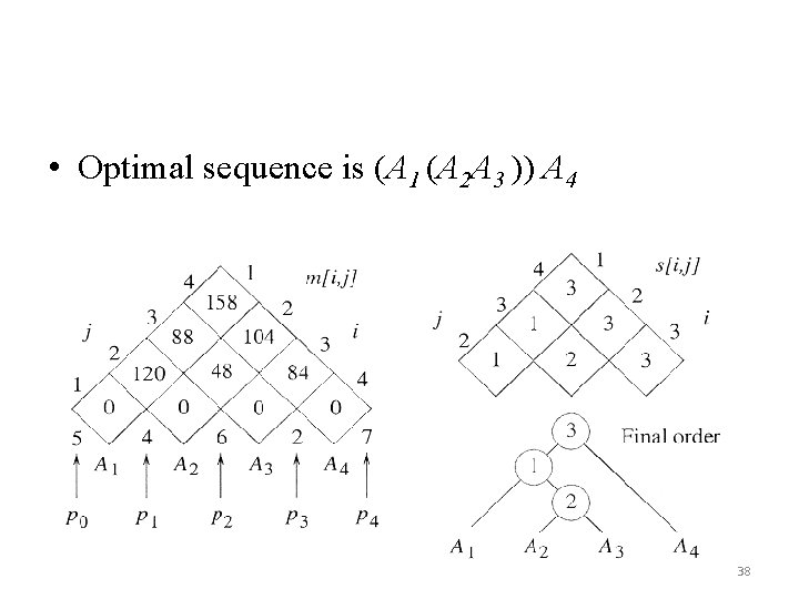
• Optimal sequence is (A 1 (A 2 A 3 )) A 4 38

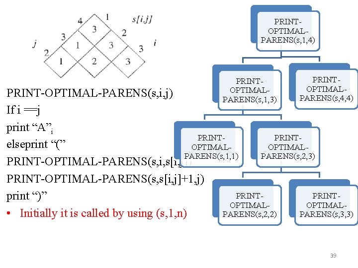
PRINTOPTIMALPARENS(s, 1, 4) PRINTOPTIMALPARENS(s, 1, 3) PRINTOPTIMALPARENS(s, 4, 4) PRINT-OPTIMAL-PARENS(s, i, j) If i ==j print “A”i PRINTelseprint “(” OPTIMALPARENS(s, 1, 1) PARENS(s, 2, 3) PRINT-OPTIMAL-PARENS(s, i, s[i, j]) PRINT-OPTIMAL-PARENS(s, s[i, j]+1, j) PRINTprint “)” OPTIMAL • Initially it is called by using (s, 1, n) PARENS(s, 2, 2) PARENS(s, 3, 3) 39

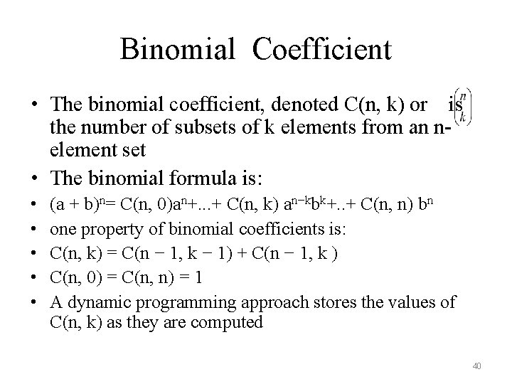
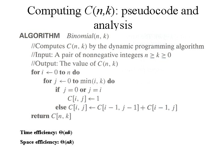
Binomial Coefficient • The binomial coefficient, denoted C(n, k) or is the number of subsets of k elements from an nelement set • The binomial formula is: • • • (a + b)n= C(n, 0)an+. . . + C(n, k) an−kbk+. . + C(n, n) bn one property of binomial coefficients is: C(n, k) = C(n − 1, k − 1) + C(n − 1, k ) C(n, 0) = C(n, n) = 1 A dynamic programming approach stores the values of C(n, k) as they are computed 40

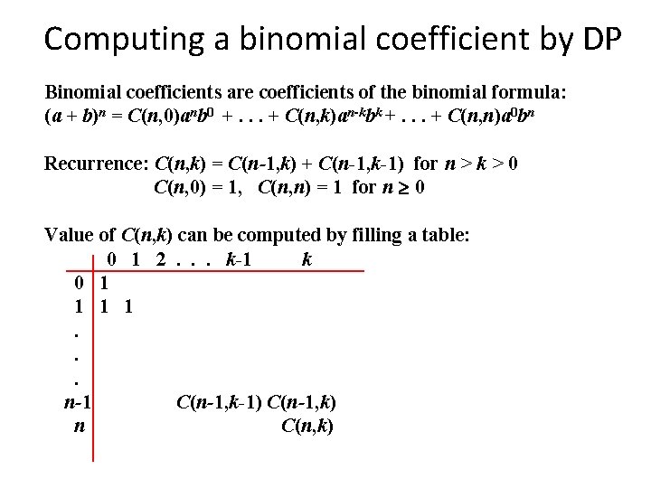
Computing a binomial coefficient by DP Binomial coefficients are coefficients of the binomial formula: (a + b)n = C(n, 0)anb 0 +. . . + C(n, k)an-kbk +. . . + C(n, n)a 0 bn Recurrence: C(n, k) = C(n-1, k) + C(n-1, k-1) for n > k > 0 C(n, 0) = 1, C(n, n) = 1 for n 0 Value of C(n, k) can be computed by filling a table: 0 1 2. . . k-1 k 0 1 1. . . n-1 C(n-1, k-1) C(n-1, k) n C(n, k)

Computing C(n, k): pseudocode and analysis Time efficiency: Θ(nk) Space efficiency: Θ(nk)

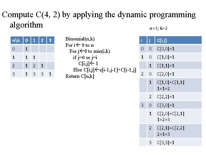
Compute C(4, 2) by applying the dynamic programming algorithm n=3; k=2 nk 0 1 2 0 1 1 2 1 3 1 3 3 3 1 Binomial(n, k) For i 0 to n For j 0 to min(i, k) if j=0 or j=i C[i, j] 1 Else C[i, j] c[i-1, j-1]+C[i-1, j] Return C[n, k] i j C[i, j] 0 0 C[0, 0]=1 1 0 C[1, 0]=1 1 C[1, 1]=1 0 C[2, 0]=1 1 C[1, 0]+C[1, 1] 1+1=2 2 C[2, 2]=1 0 C[3, 0]=1 1 C[2, 0]+C[2, 1] 1+2=3 2 C[2, 1]+C[2, 2] 2+1=3 2 3 3 C[3, 3]=1 43