UNIT II DIVIDE AND CONQUER GREEDY METHOD Design

UNIT - II DIVIDE AND CONQUER & GREEDY METHOD Design and Analysis of Algorithms - Unit II 1

Divide and Conquer The most well known algorithm design strategy: 1. Divide instance of problem into two or more smaller instances 2. Solve smaller instances recursively 3. Obtain solution to original (larger) instance by combining these solutions Design and Analysis of Algorithms - Unit II 2

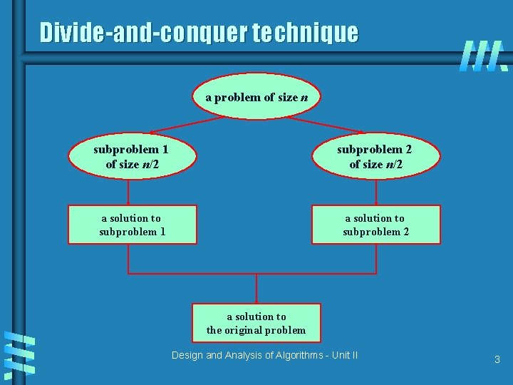
Divide-and-conquer technique a problem of size n subproblem 1 of size n/2 subproblem 2 of size n/2 a solution to subproblem 1 a solution to subproblem 2 a solution to the original problem Design and Analysis of Algorithms - Unit II 3

Divide and Conquer Examples b Sorting: mergesort and quicksort b Tree traversals b Binary search b Matrix multiplication-Strassen’s algorithm b Convex hull-Quick. Hull algorithm Design and Analysis of Algorithms - Unit II 4

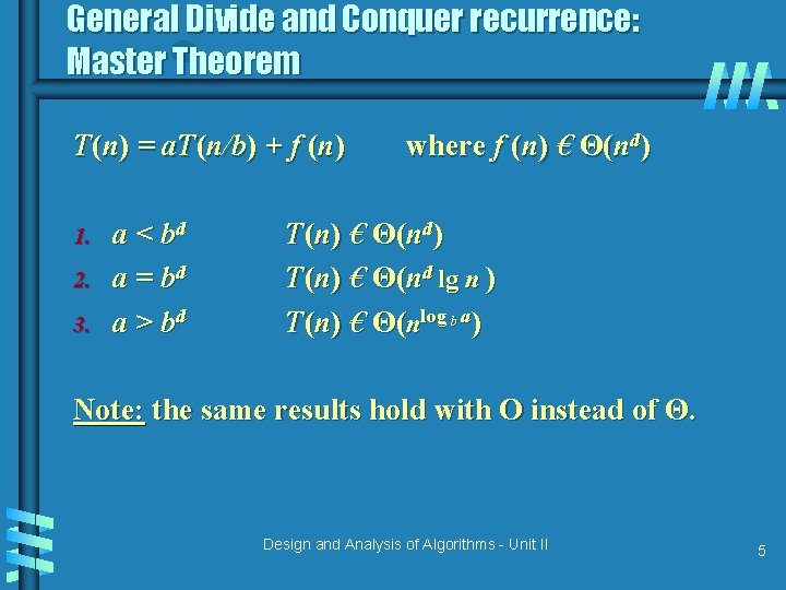
General Divide and Conquer recurrence: Master Theorem T(n) = a. T(n/b) + f (n) 1. 2. 3. a < bd a = bd a > bd where f (n) € Θ(nd) T(n) € Θ(nd lg n ) T(n) € Θ(nlog b a) Note: the same results hold with O instead of Θ. Design and Analysis of Algorithms - Unit II 5

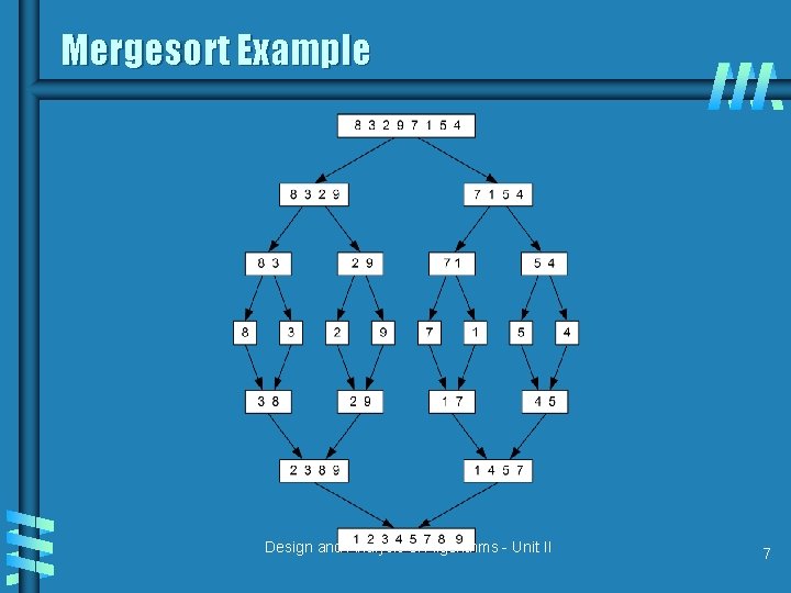
Mergesort Algorithm: b Split array A[1. . n] in two and make copies of each half in arrays B[1. . n/2 ] and C[1. . n/2 ] b Sort arrays B and C b Merge sorted arrays B and C into array A as follows: • Repeat the following until no elements remain in one of the arrays: – compare the first elements in the remaining unprocessed portions of the arrays – copy the smaller of the two into A, while incrementing the index indicating the unprocessed portion of that array • Once all elements in one of the arrays are processed, copy the remaining unprocessed elements from the other array into A. Design and Analysis of Algorithms - Unit II 6

Mergesort Example Design and Analysis of Algorithms - Unit II 7

Pseudocode for Mergesort ALGORITHM Mergesort(A[0. . n-1]) //Sorts array A[0. . n-1] by recursive mergesort // Input: An array A[0. . n-1] of orderable elements // Output: Array A[0. . n-1] sorted in non-increasing order If n>1 copy A[0. . [n/2]-1] to B[0. . [n/2]-1] copy A[[n/2]. . n-1] to C[0. . [n/2]-1] Mergesort(B[0. . [n/2]-1]) Mergesort(C[0. . [n/2]-1]) Merge(B, C, A) Design and Analysis of Algorithms - Unit II 8

Pseudocode for Merge ALGORITHM Merge (B[0. . p-1], C[0. . q-1], A[0. . p+q-1] // Merges two sorted arrays into one sorted array // Input: Arrays B[0. . p-1] and C[0. . q-1] both sorted // Output: Sorted array A[0. . p+q-1] of the elements of B and C i 0; j 0; k 0 While i<p and j<q do if B[i]<=C[j] A[k] B[i]; i i+1 else A[k] C[j]; j j+1 k k+1 If i=p copy C[j. . q-1] to A[k. . p+q-1] Else copy B[i. . p-1] to A[k. . p+q-1] Design and Analysis of Algorithms - Unit II 9

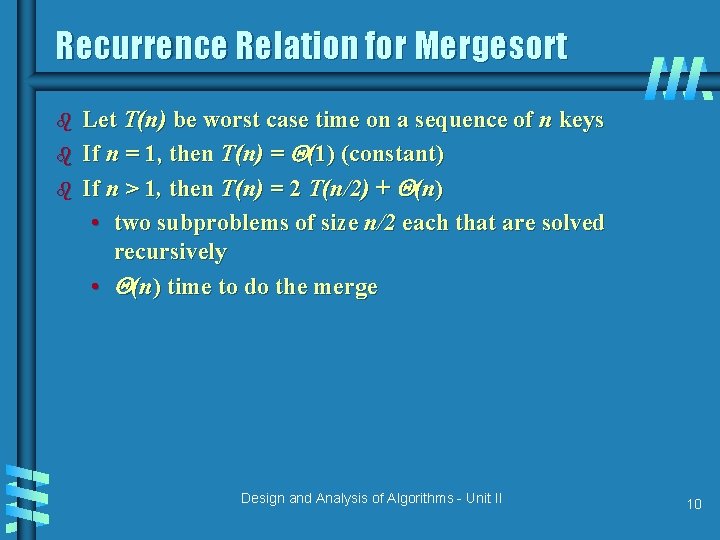
Recurrence Relation for Mergesort b b b Let T(n) be worst case time on a sequence of n keys If n = 1, then T(n) = (1) (constant) If n > 1, then T(n) = 2 T(n/2) + (n) • two subproblems of size n/2 each that are solved recursively • (n) time to do the merge Design and Analysis of Algorithms - Unit II 10

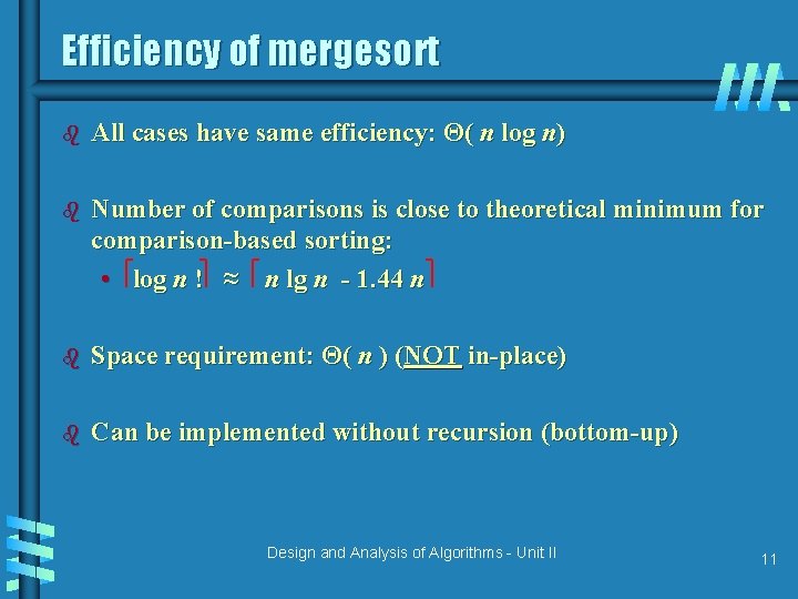
Efficiency of mergesort b All cases have same efficiency: Θ( n log n) b Number of comparisons is close to theoretical minimum for comparison-based sorting: • log n ! ≈ n lg n - 1. 44 n b Space requirement: Θ( n ) (NOT in-place) b Can be implemented without recursion (bottom-up) Design and Analysis of Algorithms - Unit II 11

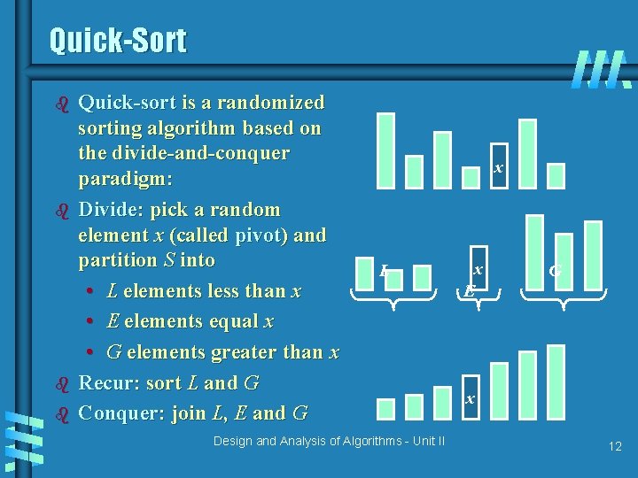
Quick-Sort b b Quick-sort is a randomized sorting algorithm based on the divide-and-conquer paradigm: Divide: pick a random element x (called pivot) and partition S into • L elements less than x • E elements equal x • G elements greater than x Recur: sort L and G Conquer: join L, E and G x L Design and Analysis of Algorithms - Unit II x E G x 12

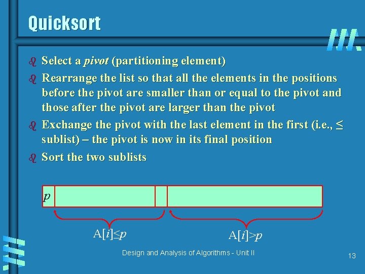
Quicksort b b Select a pivot (partitioning element) Rearrange the list so that all the elements in the positions before the pivot are smaller than or equal to the pivot and those after the pivot are larger than the pivot Exchange the pivot with the last element in the first (i. e. , ≤ sublist) – the pivot is now in its final position Sort the two sublists p A[i]≤p A[i]>p Design and Analysis of Algorithms - Unit II 13

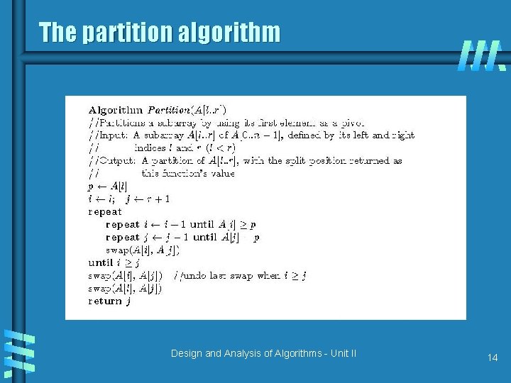
The partition algorithm Design and Analysis of Algorithms - Unit II 14

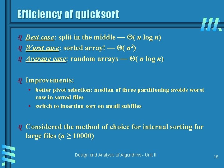
Efficiency of quicksort b Best case: split in the middle — Θ( n log n) Worst case: sorted array! — Θ( n 2) Average case: random arrays — Θ( n log n) b Improvements: b b • better pivot selection: median of three partitioning avoids worst case in sorted files • switch to insertion sort on small subfiles b Considered the method of choice for internal sorting for large files (n ≥ 10000) Design and Analysis of Algorithms - Unit II 15

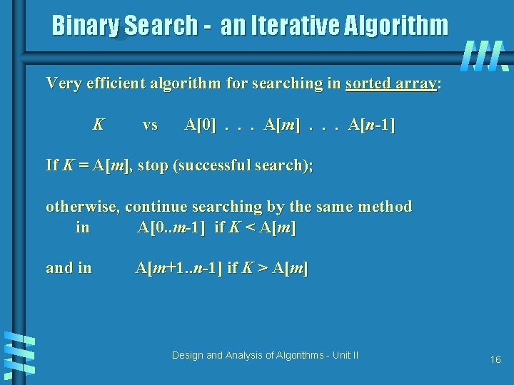
Binary Search - an Iterative Algorithm Very efficient algorithm for searching in sorted array: K vs A[0]. . . A[m]. . . A[n-1] If K = A[m], stop (successful search); otherwise, continue searching by the same method in A[0. . m-1] if K < A[m] and in A[m+1. . n-1] if K > A[m] Design and Analysis of Algorithms - Unit II 16

Pseudocode for Binary Search ALGORITHM Binary. Search(A[0. . n-1], K) l 0; r n-1 while l r do // l and r crosses over can’t find K m (l+r)/2 if K = A[m] return m //the key is found else if K < A[m] r m-1 //the key is on the left half of the array else l m+1 // the key is on the right half of the array return -1 Design and Analysis of Algorithms - Unit II 17

Binary Search – a Recursive Algorithm ALGORITHM Binary. Search. Recur(A[0. . n-1], l, r, K) if l > r return – 1 else m (l + r) / 2 if K = A[m] return m else if K < A[m] return Binary. Search. Recur(A[0. . n-1], l, m-1, K) else return Binary. Search. Recur(A[0. . n-1], m+1, r, K) Design and Analysis of Algorithms - Unit II 18

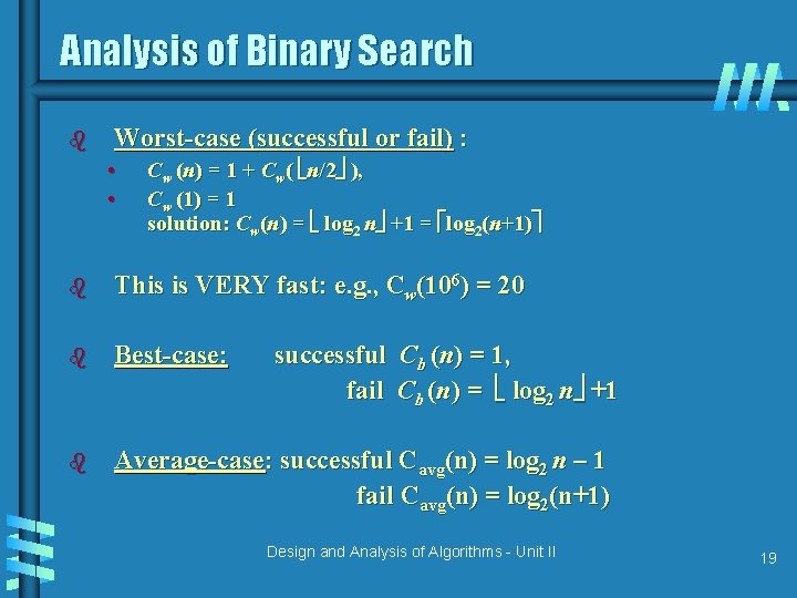
Analysis of Binary Search b Worst-case (successful or fail) : • • Cw (n) = 1 + Cw( n/2 ), Cw (1) = 1 solution: Cw(n) = log 2 n +1 = log 2(n+1) b This is VERY fast: e. g. , Cw(106) = 20 b Best-case: b Average-case: successful Cavg(n) = log 2 n – 1 fail Cavg(n) = log 2(n+1) successful Cb (n) = 1, fail Cb (n) = log 2 n +1 Design and Analysis of Algorithms - Unit II 19

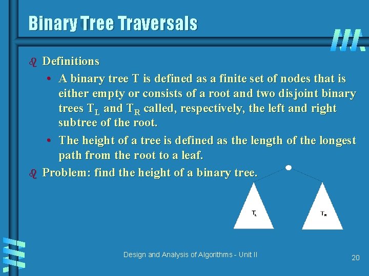
Binary Tree Traversals b b Definitions • A binary tree T is defined as a finite set of nodes that is either empty or consists of a root and two disjoint binary trees TL and TR called, respectively, the left and right subtree of the root. • The height of a tree is defined as the length of the longest path from the root to a leaf. Problem: find the height of a binary tree. Design and Analysis of Algorithms - Unit II 20

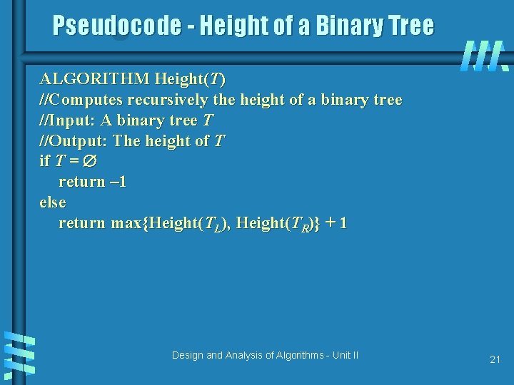
Pseudocode - Height of a Binary Tree ALGORITHM Height(T) //Computes recursively the height of a binary tree //Input: A binary tree T //Output: The height of T if T = return – 1 else return max{Height(TL), Height(TR)} + 1 Design and Analysis of Algorithms - Unit II 21

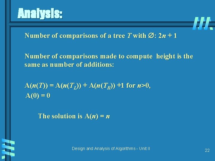
Analysis: Number of comparisons of a tree T with : 2 n + 1 Number of comparisons made to compute height is the same as number of additions: A(n(T)) = A(n(TL)) + A(n(TR)) +1 for n>0, A(0) = 0 The solution is A(n) = n Design and Analysis of Algorithms - Unit II 22

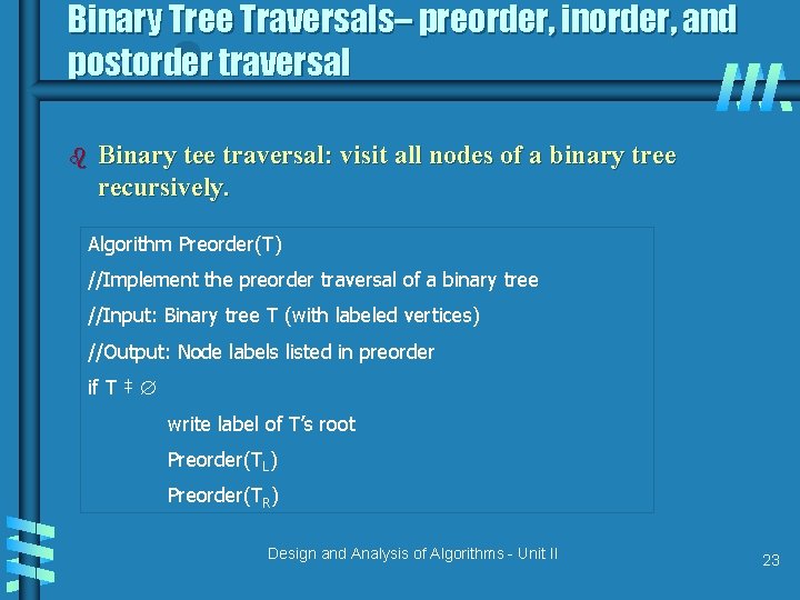
Binary Tree Traversals– preorder, inorder, and postorder traversal b Binary tee traversal: visit all nodes of a binary tree recursively. Algorithm Preorder(T) //Implement the preorder traversal of a binary tree //Input: Binary tree T (with labeled vertices) //Output: Node labels listed in preorder if T ‡ write label of T’s root Preorder(TL) Preorder(TR) Design and Analysis of Algorithms - Unit II 23

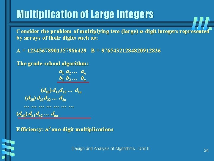
Multiplication of Large Integers Consider the problem of multiplying two (large) n-digit integers represented by arrays of their digits such as: A = 12345678901357986429 B = 87654321284820912836 The grade-school algorithm: a 1 a 2 … an b 1 b 2 … bn (d 10) d 11 d 12 … d 1 n (d 20) d 21 d 22 … d 2 n ………………… (dn 0) dn 1 dn 2 … dnn Efficiency: n 2 one-digit multiplications Design and Analysis of Algorithms - Unit II 24

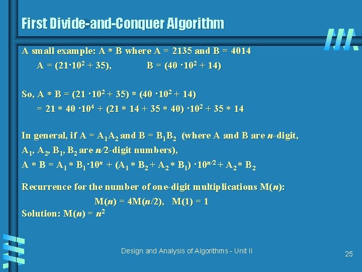
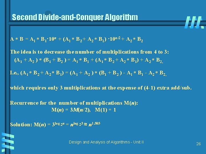
First Divide-and-Conquer Algorithm A small example: A B where A = 2135 and B = 4014 A = (21· 102 + 35), B = (40 · 102 + 14) So, A B = (21 · 102 + 35) (40 · 102 + 14) = 21 40 · 104 + (21 14 + 35 40) · 102 + 35 14 In general, if A = A 1 A 2 and B = B 1 B 2 (where A and B are n-digit, A 1, A 2, B 1, B 2 are n/2 -digit numbers), A B = A 1 B 1· 10 n + (A 1 B 2 + A 2 B 1) · 10 n/2 + A 2 B 2 Recurrence for the number of one-digit multiplications M(n): M(n) = 4 M(n/2), M(1) = 1 Solution: M(n) = n 2 Design and Analysis of Algorithms - Unit II 25

Second Divide-and-Conquer Algorithm A B = A 1 B 1· 10 n + (A 1 B 2 + A 2 B 1) · 10 n/2 + A 2 B 2 The idea is to decrease the number of multiplications from 4 to 3: (A 1 + A 2 ) (B 1 + B 2 ) = A 1 B 1 + (A 1 B 2 + A 2 B 1) + A 2 B 2, I. e. , (A 1 B 2 + A 2 B 1) = (A 1 + A 2 ) (B 1 + B 2 ) - A 1 B 1 - A 2 B 2, which requires only 3 multiplications at the expense of (4 -1) extra add/sub. Recurrence for the number of multiplications M(n): M(n) = 3 M(n/2), M(1) = 1 Solution: M(n) = 3 log 2 n = nlog 23 ≈ n 1. 585 Design and Analysis of Algorithms - Unit II 26

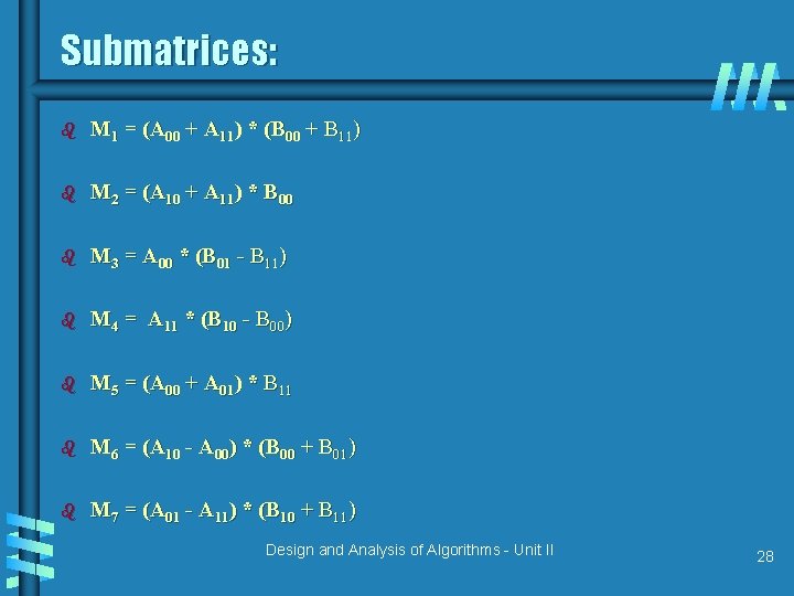
Strassen’s matrix multiplication b Strassen observed [1969] that the product of two matrices can be computed as follows: C 00 C 01 A 00 A 01 = C 10 C 11 B 00 B 01 * A 10 A 11 B 10 B 11 M 1 + M 4 - M 5 + M 7 M 3 + M 5 = M 2 + M 4 M 1 + M 3 - M 2 + M 6 Design and Analysis of Algorithms - Unit II 27

Submatrices: b M 1 = (A 00 + A 11) * (B 00 + B 11) b M 2 = (A 10 + A 11) * B 00 b M 3 = A 00 * (B 01 - B 11) b M 4 = A 11 * (B 10 - B 00) b M 5 = (A 00 + A 01) * B 11 b M 6 = (A 10 - A 00) * (B 00 + B 01) b M 7 = (A 01 - A 11) * (B 10 + B 11) Design and Analysis of Algorithms - Unit II 28

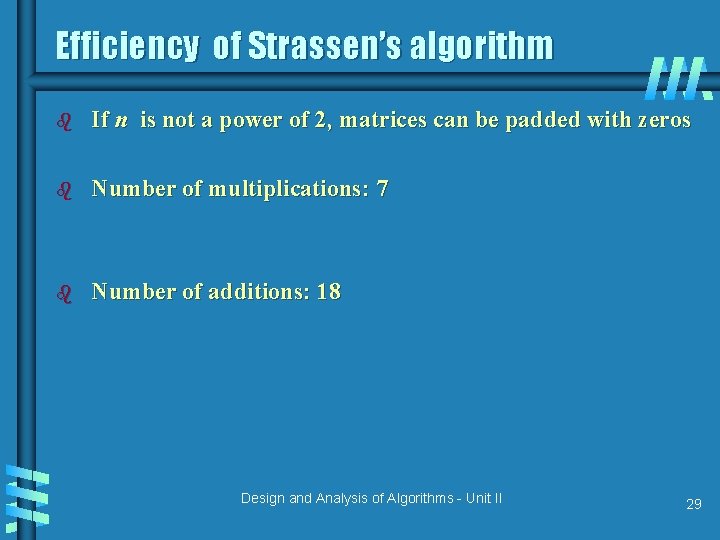
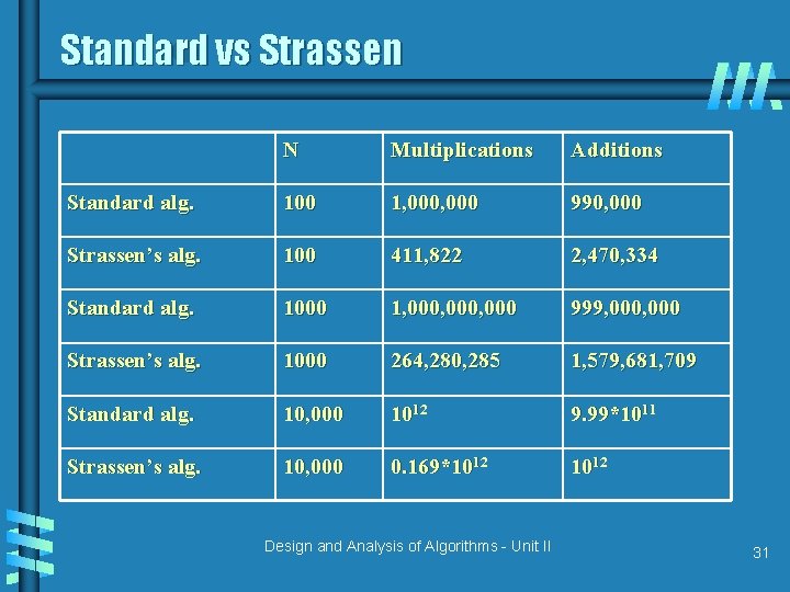
Efficiency of Strassen’s algorithm b If n is not a power of 2, matrices can be padded with zeros b Number of multiplications: 7 b Number of additions: 18 Design and Analysis of Algorithms - Unit II 29

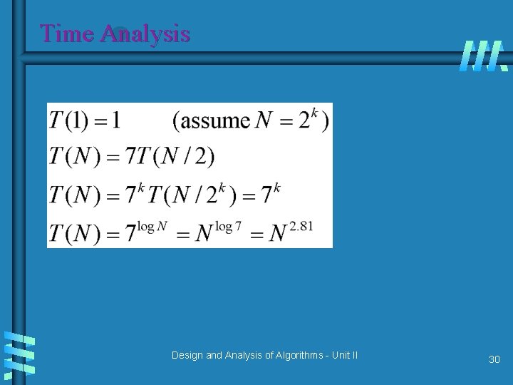
Time Analysis Design and Analysis of Algorithms - Unit II 30

Standard vs Strassen N Multiplications Additions Standard alg. 100 1, 000 990, 000 Strassen’s alg. 100 411, 822 2, 470, 334 Standard alg. 1000 1, 000, 000 999, 000 Strassen’s alg. 1000 264, 280, 285 1, 579, 681, 709 Standard alg. 10, 000 1012 9. 99*1011 Strassen’s alg. 10, 000 0. 169*1012 Design and Analysis of Algorithms - Unit II 31

Greedy Technique Design and Analysis of Algorithms - Unit II

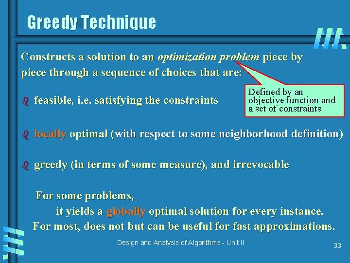
Greedy Technique Constructs a solution to an optimization problem piece by piece through a sequence of choices that are: Defined by an objective function and a set of constraints b feasible, i. e. satisfying the constraints b locally optimal (with respect to some neighborhood definition) b greedy (in terms of some measure), and irrevocable For some problems, it yields a globally optimal solution for every instance. For most, does not but can be useful for fast approximations. Design and Analysis of Algorithms - Unit II 33

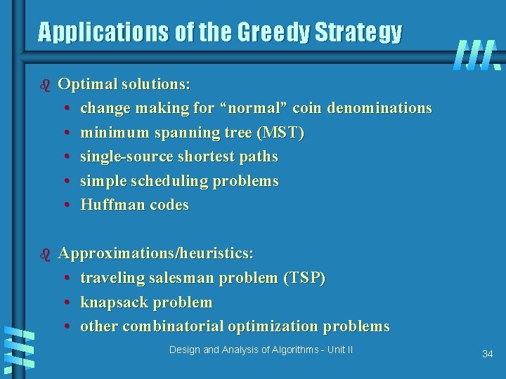
Applications of the Greedy Strategy b Optimal solutions: • change making for “normal” coin denominations • minimum spanning tree (MST) • single-source shortest paths • simple scheduling problems • Huffman codes b Approximations/heuristics: • traveling salesman problem (TSP) • knapsack problem • other combinatorial optimization problems Design and Analysis of Algorithms - Unit II 34

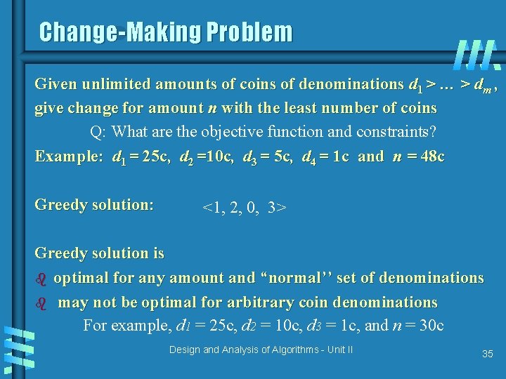
Change-Making Problem Given unlimited amounts of coins of denominations d 1 > … > dm , give change for amount n with the least number of coins Q: What are the objective function and constraints? Example: d 1 = 25 c, d 2 =10 c, d 3 = 5 c, d 4 = 1 c and n = 48 c Greedy solution: <1, 2, 0, 3> Greedy solution is b optimal for any amount and “normal’’ set of denominations b may not be optimal for arbitrary coin denominations For example, d 1 = 25 c, d 2 = 10 c, d 3 = 1 c, and n = 30 c Design and Analysis of Algorithms - Unit II 35

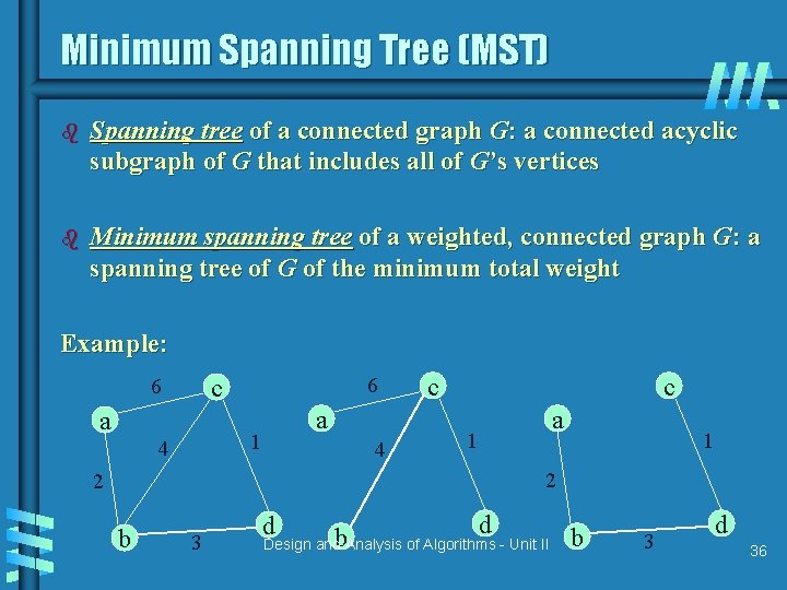
Minimum Spanning Tree (MST) b Spanning tree of a connected graph G: a connected acyclic subgraph of G that includes all of G’s vertices b Minimum spanning tree of a weighted, connected graph G: a spanning tree of G of the minimum total weight Example: 6 c 6 a a 1 4 4 c c 1 a 1 2 2 b 3 d b Design and Analysis of Algorithms - Unit II b d 36

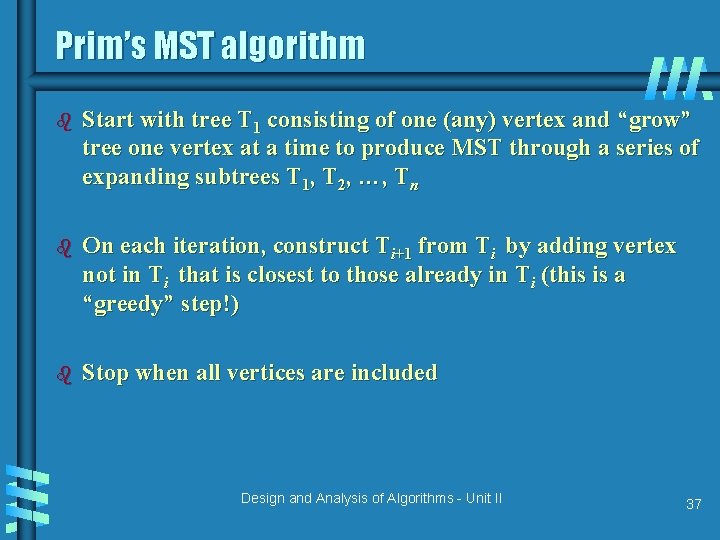
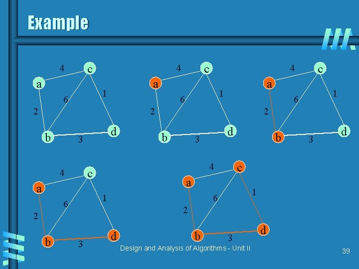
Prim’s MST algorithm b Start with tree T 1 consisting of one (any) vertex and “grow” tree one vertex at a time to produce MST through a series of expanding subtrees T 1, T 2, …, Tn b On each iteration, construct Ti+1 from Ti by adding vertex not in Ti that is closest to those already in Ti (this is a “greedy” step!) b Stop when all vertices are included Design and Analysis of Algorithms - Unit II 37

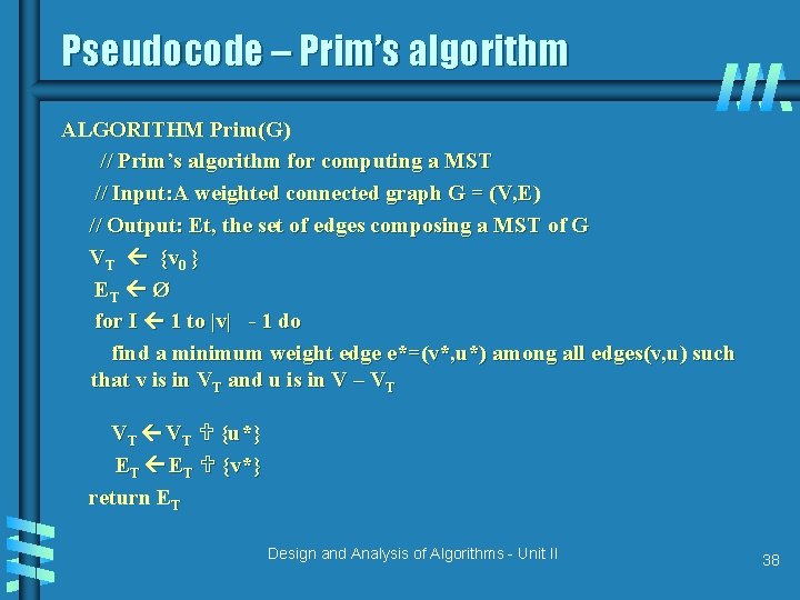
Pseudocode – Prim’s algorithm ALGORITHM Prim(G) // Prim’s algorithm for computing a MST // Input: A weighted connected graph G = (V, E) // Output: Et, the set of edges composing a MST of G VT {v 0 } ET Ø for I 1 to |v| - 1 do find a minimum weight edge e*=(v*, u*) among all edges(v, u) such that v is in VT and u is in V – VT VT {u*} ET {v*} return ET Design and Analysis of Algorithms - Unit II 38

Example c 4 a a 1 6 b d 3 a b d 3 b 3 d c a 1 6 2 2 b 2 4 c 4 1 6 2 2 c 4 a 1 6 c 4 3 d b 3 Design and Analysis of Algorithms - Unit II d 39

Notes about Prim’s algorithm b Needs priority queue for locating closest fringe vertex. b Efficiency • O(n 2) for weight matrix representation of graph and array implementation of priority queue • O(m log n) for adjacency lists representation of graph with n vertices and m edges and min-heap implementation of the priority queue Design and Analysis of Algorithms - Unit II 40

Another greedy algorithm for MST: Kruskal’s b Sort the edges in nondecreasing order of lengths b “Grow” tree one edge at a time to produce MST through a series of expanding forests F 1, F 2, …, Fn-1 b On each iteration, add the next edge on the sorted list unless this would create a cycle. (If it would, skip the edge. ) Design and Analysis of Algorithms - Unit II 41

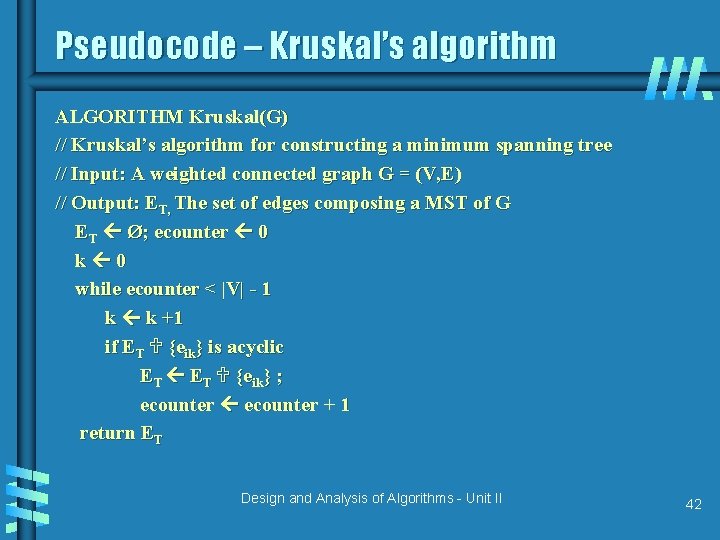
Pseudocode – Kruskal’s algorithm ALGORITHM Kruskal(G) // Kruskal’s algorithm for constructing a minimum spanning tree // Input: A weighted connected graph G = (V, E) // Output: ET, The set of edges composing a MST of G ET Ø; ecounter 0 k 0 while ecounter < |V| - 1 k k +1 if ET {eik} is acyclic ET {eik} ; ecounter + 1 return ET Design and Analysis of Algorithms - Unit II 42

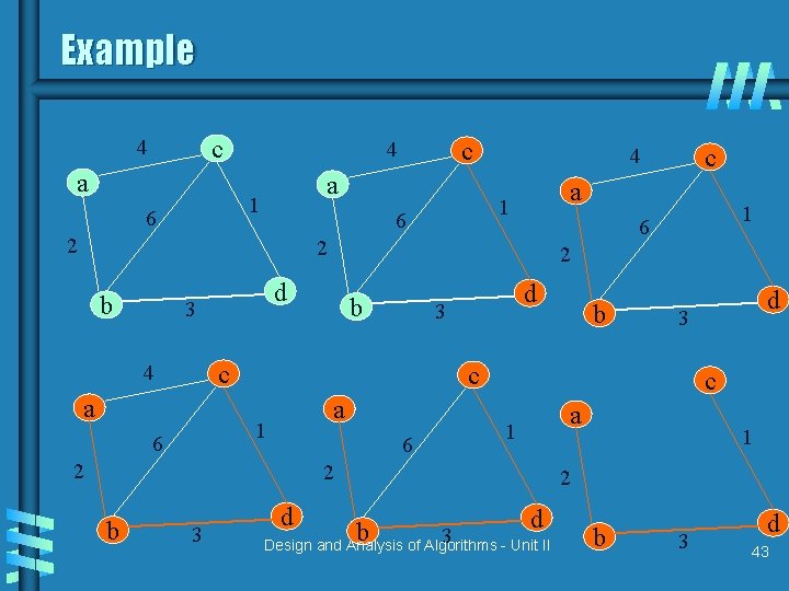
Example c 4 a a 1 6 c 4 2 a 1 6 2 d 3 b a a 6 2 3 d d 3 c 1 2 b b c 1 6 d 3 c 4 1 6 2 b c 4 d b 3 Design and Analysis of Algorithms - Unit II a 1 2 b 3 d 43

Notes about Kruskal’s algorithm b Algorithm looks easier than Prim’s but is harder to implement (checking for cycles!) b Cycle checking: a cycle is created iff added edge connects vertices in the same connected component b Kruskal’s algorithm relies on a union-find algorithm for checking cycles b Runs in O(m log m) time, with m = |E|. The time is mostly spent on sorting. Design and Analysis of Algorithms - Unit II 44

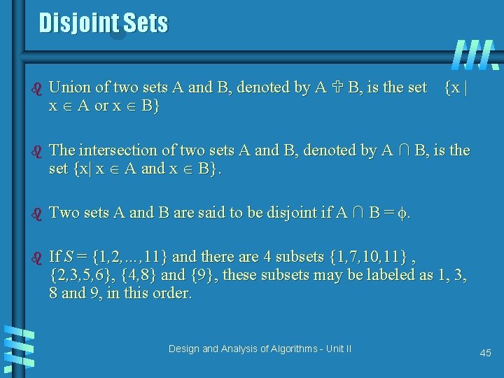
Disjoint Sets b Union of two sets A and B, denoted by A B, is the set {x | x A or x B} b The intersection of two sets A and B, denoted by A ∩ B, is the set {x| x A and x B}. b Two sets A and B are said to be disjoint if A ∩ B = . b If S = {1, 2, …, 11} and there are 4 subsets {1, 7, 10, 11} , {2, 3, 5, 6}, {4, 8} and {9}, these subsets may be labeled as 1, 3, 8 and 9, in this order. Design and Analysis of Algorithms - Unit II 45

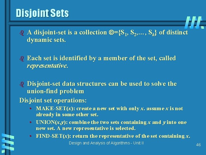
Disjoint Sets b A disjoint-set is a collection ={S 1, S 2, …, Sk} of distinct dynamic sets. b Each set is identified by a member of the set, called representative. Disjoint-set data structures can be used to solve the union-find problem Disjoint set operations: b • MAKE-SET(x): create a new set with only x. assume x is not already in some other set. • UNION(x, y): combine the two sets containing x and y into one new set. A new representative is selected. • FIND-SET(x): return the representative of the set containing x. Design and Analysis of Algorithms - Unit II 46

The Union-Find problem b N balls initially, each ball in its own bag • Label the balls 1, 2, 3, . . . , N b Two kinds of operations: • Pick two bags, put all balls in these bags into a new bag (Union) • Given a ball, find the bag containing it (Find) Design and Analysis of Algorithms - Unit II 47

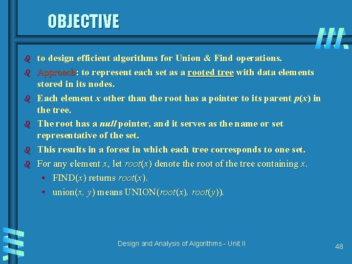
OBJECTIVE b b b to design efficient algorithms for Union & Find operations. Approach: to represent each set as a rooted tree with data elements stored in its nodes. Each element x other than the root has a pointer to its parent p(x) in the tree. The root has a null pointer, and it serves as the name or set representative of the set. This results in a forest in which each tree corresponds to one set. For any element x, let root(x) denote the root of the tree containing x. • FIND(x) returns root(x). • union(x, y) means UNION(root(x), root(y)). Design and Analysis of Algorithms - Unit II 48

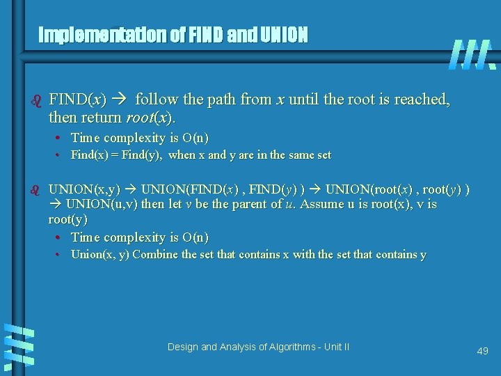
Implementation of FIND and UNION b FIND(x) follow the path from x until the root is reached, then return root(x). • Time complexity is O(n) • Find(x) = Find(y), when x and y are in the same set b UNION(x, y) UNION(FIND(x) , FIND(y) ) UNION(root(x) , root(y) ) UNION(u, v) then let v be the parent of u. Assume u is root(x), v is root(y) • Time complexity is O(n) • Union(x, y) Combine the set that contains x with the set that contains y Design and Analysis of Algorithms - Unit II 49

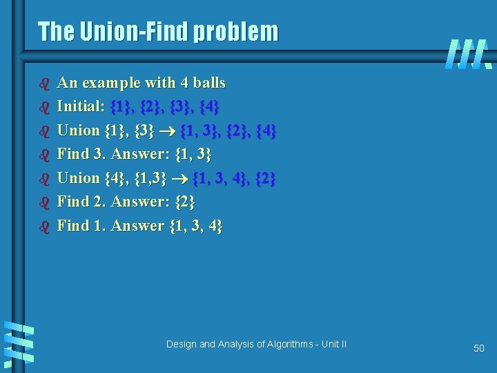
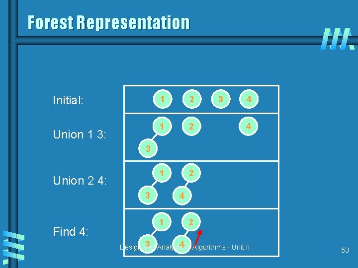
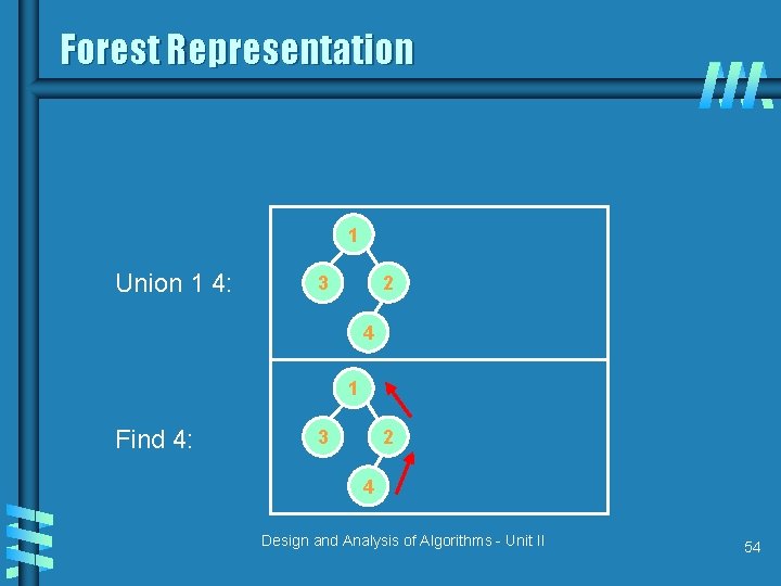
The Union-Find problem b b b b An example with 4 balls Initial: {1}, {2}, {3}, {4} Union {1}, {3} {1, 3}, {2}, {4} Find 3. Answer: {1, 3} Union {4}, {1, 3} {1, 3, 4}, {2} Find 2. Answer: {2} Find 1. Answer {1, 3, 4} Design and Analysis of Algorithms - Unit II 50

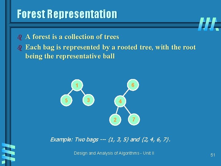
Forest Representation b b A forest is a collection of trees Each bag is represented by a rooted tree, with the root being the representative ball 6 1 5 3 4 2 7 Example: Two bags --- {1, 3, 5} and {2, 4, 6, 7}. Design and Analysis of Algorithms - Unit II 51

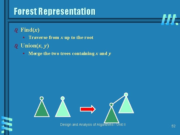
Forest Representation b Find(x) • Traverse from x up to the root b Union(x, y) • Merge the two trees containing x and y Design and Analysis of Algorithms - Unit II 52

Forest Representation Initial: Union 1 3: 1 2 1 2 3 4 4 3 Union 2 4: 3 Find 4: 4 1 2 3 Analysis 4 of Algorithms - Unit II Design and 53

Forest Representation 1 Union 1 4: 2 3 4 1 Find 4: 2 3 4 Design and Analysis of Algorithms - Unit II 54

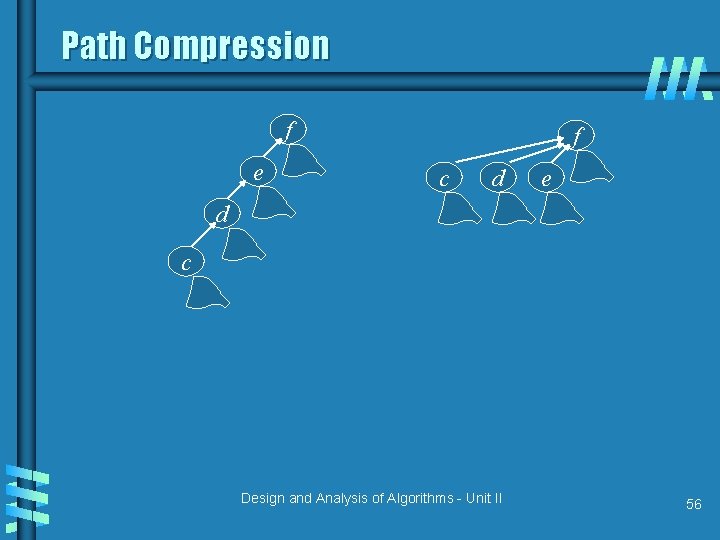
Union by Rank & Path Compression b Union by Rank: Each node is associated with a rank, which is the upper bound on the height of the node (i. e. , the height of subtree rooted at the node), then when UNION, let the root with smaller rank point to the root with larger rank. b Path Compression: used in FIND-SET(x) operation, make each node in the path from x to the root directly point to the root. Thus reduce the tree height. Design and Analysis of Algorithms - Unit II 55

Path Compression f e f c d e d c Design and Analysis of Algorithms - Unit II 56

Shortest paths – Dijkstra’s algorithm Single Source Shortest Paths Problem: Given a weighted connected (directed) graph G, find shortest paths from source vertex s to each of the other vertices Dijkstra’s algorithm: Similar to Prim’s MST algorithm, with a different way of computing numerical labels: Among vertices not already in the tree, it finds vertex u with the smallest sum dv + w(v, u) where v is a vertex for which shortest path has been already found on preceding iterations (such vertices form a tree rooted at s) dv is the length of the shortest path from source s to v w(v, u) is the length (weight) of edge from v to u Design and Analysis of Algorithms - Unit II 57

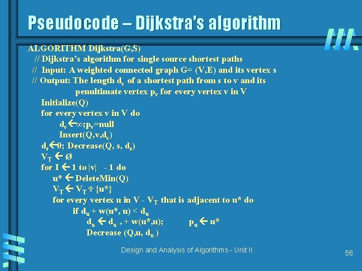
Pseudocode – Dijkstra’s algorithm ALGORITHM Dijkstra(G, S) // Dijkstra’s algorithm for single source shortest paths // Input: A weighted connected graph G= (V, E) and its vertex s // Output: The length dv of a shortest path from s to v and its penultimate vertex pv for every vertex v in V Initialize(Q) for every vertex v in V do dv ∞; pv=null Insert(Q, v, dv) ds 0; Decrease(Q, s, ds) VT Ø for I 1 to |v| - 1 do u* Delete. Min(Q) VT {u*} for every vertex u in V - VT that is adjacent to u* do if du + w(u*, u) < du du * + w(u*, u); pu u* Decrease (Q, u, du ) Design and Analysis of Algorithms - Unit II 58

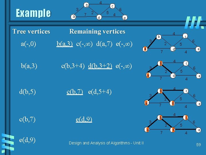
Example Tree vertices a(-, 0) b(a, 3) 3 a 4 b 7 2 c 5 d 4 6 e Remaining vertices b(a, 3) c(-, ∞) d(a, 7) e(-, ∞) 3 a c(b, 3+4) d(b, 3+2) e(-, ∞) 3 c(b, 7) e(d, 5+4) e(d, 9) a e(d, 9) Design and Analysis of Algorithms - Unit II 6 5 c 6 5 d e 4 4 2 7 c d b e 4 4 7 6 5 2 3 c d b a c(b, 7) 2 7 a d(b, 5) 4 b 4 e 59

Notes on Dijkstra’s algorithm b Doesn’t work for graphs with negative weights (whereas Floyd’s algorithm does, as long as there is no negative cycle). b Applicable to both undirected and directed graphs b Efficiency • O(|V|2) for graphs represented by weight matrix and array implementation of priority queue • O(|E|log|V|) for graphs represented by adj. lists and minheap implementation of priority queue Design and Analysis of Algorithms - Unit II 60