UNIT I ITERATIVE AND RECURSIVE ALGORITHMS Iterative Algorithms

UNIT I ITERATIVE AND RECURSIVE ALGORITHMS Iterative Algorithms: Measures of Progress and Loop Invariants-Paradigm Shift: Sequence of Actions versus Sequence of Assertions- Steps to Develop an Iterative Algorithm-Different Types of Iterative Algorithms-Typical Errors-Recursion-Forward versus Backward- Towers of Hanoi-Checklist for Recursive Algorithms-The Stack Frame-Proving Correctness with Strong Induction- Examples of Recursive Algorithms-Sorting and Selecting Algorithms. Operations on Integers Ackermann’s Function- Recursion on Trees-Tree Traversals. Examples- Generalizing the Problem -Heap Sort and Priority Queues-Representing Expressions. IFETCE/M. E(CSE)/I YEAR/I SEM/ADS/UNIT-I/PPT/VER 1. 2 1

Iterative Algorithms: Measures of Progress and Loop Invariants • An iterative algorithm to solve a computational problem is a bit like following a road, possibly long and difficult, from your start location to your destination. • With each iteration, you have a method that takes you a single step closer. • To ensure that you move forward, you need to have a measure of progress telling you how far you are either from your starting location or from your destination. IFETCE/M. E(CSE)/I YEAR/I SEM/ADS/UNIT-I/PPT/VER 1. 2 2

• You cannot expect to know exactly where the algorithm will go, so you need to expect some weaving and winding. • On the other hand, you do not want to have to know how to handle every ditch and dead end in the world. • A compromise between these two is to have a loop invariant, which defines a road (or region) that you may not leave. • As you travel, worry about one step at a time. IFETCE/M. E(CSE)/IYEAR/I SEM/ADS/UNIT-I/PPT/VER 1. 2 3

• You must know how to get onto the road from any start location. • From every place along the road, you must know what actions you will take in order to step forward while not leaving the road. • Finally, when sufficient progress has been made along the road, you must know how to exit and reach your destination in a reasonable amount of time. IFETCE/M. E(CSE)/IYEAR/I SEM/ADS/UNIT-I/PPT/VER 1. 2 4

A Paradigm Shift: A Sequence of Actions vs a Sequence of Assertions • Iterative algorithms requires understanding the difference between a loop invariant, which is an assertion or picture of the computation at a particular point in time, and the actions that are required to maintain such a loop invariant. • One of the first important paradigm shifts that programmers struggle to make is from viewing an algorithm as a sequence of actions to viewing it as a sequence of snapshots of the state of the computer. IFETCE/M. E(CSE)/I YEAR/I SEM/ADS/UNIT-I/PPT/VER 1. 2 5

• Programmers tend to fixate on the first view, because code is a sequence of instructions for action and a computation is a sequence of actions. • Imagine stopping time at key points during the computation and taking still pictures of the state of the computer. • Then a computation can equally be viewed as a sequence of such snapshots. • Having two ways of viewing the same thing gives one both more tools to handle it and a deeper understanding of it. IFETCE/M. E(CSE)/I YEAR/I SEM/ADS/UNIT-I/PPT/VER 1. 2 6

The Challenge of the Sequence-of-Actions View • Suppose one is designing a new algorithm or explaining an algorithm to a friend. • If one is thinking of it as sequence of actions, then one will likely start at the beginning: Do this. Do that. Do this. • Shortly one can get lost and not know where one is. • To handle this, one simultaneously needs to keep track of how the state of the computer changes with each new action. IFETCE/M. E(CSE)/I YEAR/I SEM/ADS/UNIT-I/PPT/VER 1. 2 7

• In order to know what action to take next, one needs to have a global plan of where the computation is to go. • To make it worse, the computation has many IFs and LOOPS so one has to consider all the various paths that the computation may take. Advantages of the Sequence of Snapshots View: • This new paradigm is useful one from which one can think about, explain, or develop an algorithm. IFETCE/M. E(CSE)/I YEAR/I SEM/ADS/UNIT-I/PPT/VER 1. 2 8

Steps to Develop an Iterative Algorithms: • A good way to structure many computer programs is to store the key information you currently know in some data structure • And then have each iteration of the main loop take a step towards your destination by making a simple change to this data. IFETCE/M. E(CSE)/I YEAR/I SEM/ADS/UNIT-I/PPT/VER 1. 2 9

Loop Invariant: • A loop invariant expresses important relationships among the variables that must be true at the start of every iteration and when the loop terminates. • If it is true, then the computation is still on the road. • If it is false, then the algorithm has failed. IFETCE/M. E(CSE)/I YEAR/I SEM/ADS/UNIT-I/PPT/VER 1. 2 10

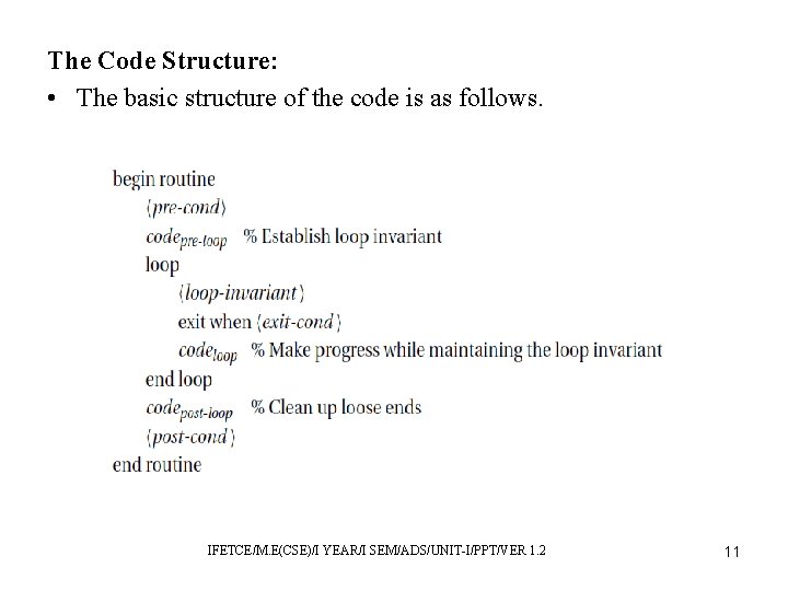
The Code Structure: • The basic structure of the code is as follows. IFETCE/M. E(CSE)/I YEAR/I SEM/ADS/UNIT-I/PPT/VER 1. 2 11

Proof of Correctness: • Naturally, you want to be sure your algorithm will work on all specified inputs and give the correct answer. Running Time: • You also want to be sure that your algorithm completes in a reasonable amount of time. The Most Important Steps: • If you need to design an algorithm, do not start by typing in code without really knowing how or why the algorithm works. • Instead, first accomplishing the following tasks. IFETCE/M. E(CSE)/I YEAR/I SEM/ADS/UNIT-I/PPT/VER 1. 2 12

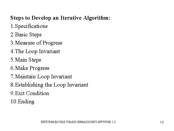
Steps to Develop an Iterative Algorithm: 1. Specifications 2. Basic Steps 3. Measure of Progress 4. The Loop Invariant 5. Main Steps 6. Make Progress 7. Maintain Loop Invariant 8. Establishing the Loop Invariant 9. Exit Condition 10. Ending IFETCE/M. E(CSE)/I YEAR/I SEM/ADS/UNIT-I/PPT/VER 1. 2 13

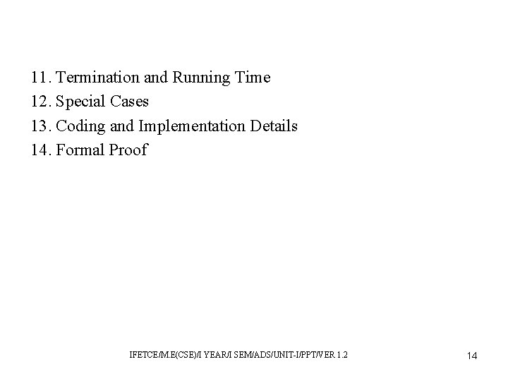
11. Termination and Running Time 12. Special Cases 13. Coding and Implementation Details 14. Formal Proof IFETCE/M. E(CSE)/I YEAR/I SEM/ADS/UNIT-I/PPT/VER 1. 2 14

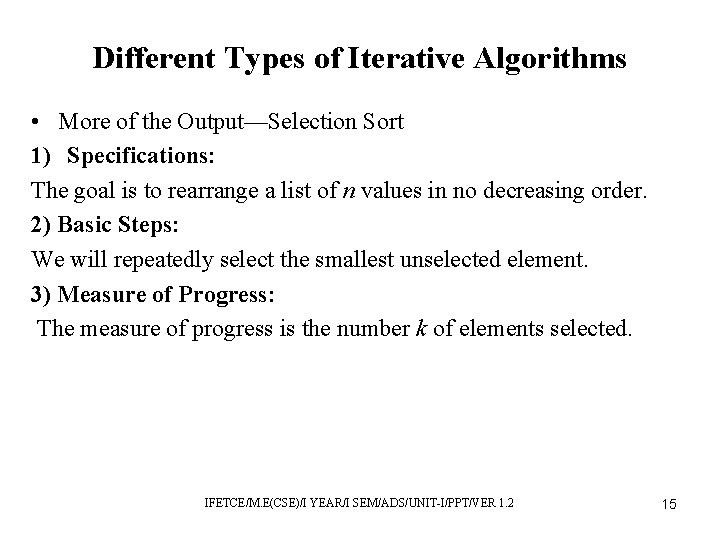
Different Types of Iterative Algorithms • More of the Output—Selection Sort 1) Specifications: The goal is to rearrange a list of n values in no decreasing order. 2) Basic Steps: We will repeatedly select the smallest unselected element. 3) Measure of Progress: The measure of progress is the number k of elements selected. IFETCE/M. E(CSE)/I YEAR/I SEM/ADS/UNIT-I/PPT/VER 1. 2 15

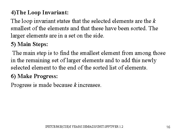
4)The Loop Invariant: The loop invariant states that the selected elements are the k smallest of the elements and that these have been sorted. The larger elements are in a set on the side. 5) Main Steps: The main step is to find the smallest element from among those in the remaining set of larger elements and to add this newly selected element to the end of the sorted list of elements. 6) Make Progress: Progress is made because k increases. IFETCE/M. E(CSE)/I YEAR/I SEM/ADS/UNIT-I/PPT/VER 1. 2 16

7) Maintain Loop Invariant: • We must prove that loop-invariant & not exit−cond & codeloop ⇒ loop-invariant. • By the previous loop invariant, the newly selected element is at least the size of the previously selected elements. • By the step, it is no bigger than the elements on the side. • It follows that it must be the k + 1 st element in the list. • Hence, moving this element from the set on the side to the end of the sorted list ensures that the selected elements in the new list are the k + 1 smallest and are sorted. IFETCE/M. E(CSE)/I YEAR/I SEM/ADS/UNIT-I/PPT/VER 1. 2 17

8) Establishing the Loop Invariant: We must prove that precond & codepre-loop ⇒loop-invariant Initially, k = 0 are sorted and all the elements are set aside. 9) Exit Condition: Stop when k = n. 10) Ending: We must prove loop-invariant & exit-cond & codepost-loop ⇒post-cond. By the exit condition, all the elements have been selected, and by the loop invariant these selected elements have been sorted. IFETCE/M. E(CSE)/I YEAR/I SEM/ADS/UNIT-I/PPT/VER 1. 2 18

11) Termination and Running Time: We have not considered how long it takes to find the next smallest element or to handle the data structures. Typical Errors: Be Clear: • The code specifies the current subinterval A[i. . j ]with two integers i and j. • Clearly document whether the sublist includes the end points i and j or not. It does not matter which, but you must be consistent. Confusion in details like this is the cause of many bugs. IFETCE/M. E(CSE)/I YEAR/I SEM/ADS/UNIT-I/PPT/VER 1. 2 19

Math Details: • Small math operations like computing the index of the middle element of the subinterval A(i. . j ) are prone to bugs. • Check for yourself that the answer is mid = [i+j/2] IFETCE/M. E(CSE)/I YEAR/I SEM/ADS/UNIT-I/PPT/VER 1. 2 20

Recursion-Forward versus Backward Recursion • Recursion is more than just a programming technique. It has two other uses in computer science and software engineering, namely: • a way of describing, defining, or specifying things. • a way of designing solutions to problems (divide and conquer). IFETCE/M. E(CSE)/I YEAR/I SEM/ADS/UNIT-I/PPT/VER 1. 2 21

Stack of Stack Frames: • Recursive algorithms are executed using a stack of stackframes. Tree of Stack Frames: • This is a useful way of viewing the entire computation at once. • It is particularly useful when computing the running time of the algorithm. • However, the structure of the computation tree may be very complex and difficult to understand all at once. IFETCE/M. E(CSE)/IYEAR/I SEM/ADS/UNIT-I/PPT/VER 1. 2 22

Friends, on Strong Induction: • You construct for each friend an instance of the same computational problem that is smaller then your own. This is referred as subinstances. • Your friends magically provide you with the solutions to these. • You then combine these subsolutions into a solution for your original instance. • I refer to this as the friends level of abstraction. • If you prefer, you can call it the strong induction level of abstraction and use the word “recursion” instead of “friend. ” IFETCE/M. E (CSE)/I YEAR/I SEM/ADS/UNIT-I/PPT/VER 1. 2 23

Forward vs. Backward • Recursion involves designing an algorithm by using it as if it already exists. At first this looks paradoxical. • Suppose, for example, the key to the • house that you want to get into is in that same house. If you could get in, you could get the key. • Then you could open the door, so that you could get in. This is a circular argument. • It is not a legal recursive program because the subinstance is not smaller. IFETCE/M. E(CSE)/I YEAR/I SEM/ADS/UNIT-I/PPT/VER 1. 2 24

Working Forward vs. Backward • An iterative algorithm works forward. • It knows about house i − 1. It uses a loop invariant to show that this house has been opened. • It searches this house and learns that the key within it is that for house i. • Because of this, it decides that house i would be a good one to go to next. IFETCE/M. E(CSE)/I YEAR/I SEM/ADS/UNIT-I/PPT/VER 1. 2 25

• A recursion algorithm works backward. It knows about house i. It wants to get it open. • It determines that the key for house i is contained in house i − 1. • Hence, opening house i − 1 is a subtask that needs to be accomplished. Advantages of recursive algorithms over iterative ones: • The first is that sometimes it is easier to work backward than forward. • The second is that a recursive algorithm is allowed to have more than one subtask to be solved. • This forms a tree of houses to open instead of a row of houses. IFETCE/M. E(CSE)/I YEAR/I SEM/ADS/UNIT-I/PPT/VER 1. 2 26

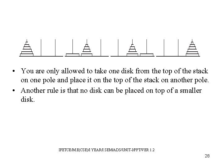
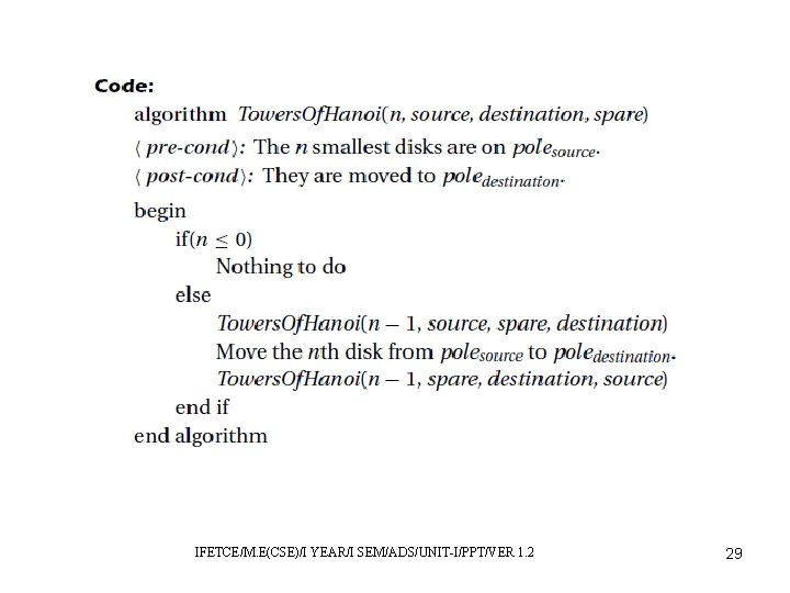
Towers of Hanoi • The towers of Hanoi is a classic puzzle for which the only possible way of solving it is to think recursively. • Specification: The puzzle consists of three poles and a stack of N disks of different sizes. • Precondition: All the disks are on the first of the three poles. • Postcondition: The goal is to move the stack over to the last pole. See the first and the last parts of figure. IFETCE/M. E(CSE)/I YEAR/I SEM/ADS/UNIT-I/PPT/VER 1. 2 27

• You are only allowed to take one disk from the top of the stack on one pole and place it on the top of the stack on another pole. • Another rule is that no disk can be placed on top of a smaller disk. IFETCE/M. E(CSE)/I YEAR/I SEM/ADS/UNIT-I/PPT/VER 1. 2 28

IFETCE/M. E(CSE)/I YEAR/I SEM/ADS/UNIT-I/PPT/VER 1. 2 29

Checklist for Recursive Algorithms • Writing a recursive algorithm is surprisingly hard when you are first starting out and surprisingly easy when you get it. • This section contains a list of things to think about to make sure that you do not make any of the common mistakes. IFETCE/M. E(CSE)/I YEAR/I SEM/ADS/UNIT-I/PPT/VER 1. 2 30

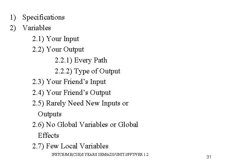
1) Specifications 2) Variables 2. 1) Your Input 2. 2) Your Output 2. 2. 1) Every Path 2. 2. 2) Type of Output 2. 3) Your Friend’s Input 2. 4) Your Friend’s Output 2. 5) Rarely Need New Inputs or Outputs 2. 6) No Global Variables or Global Effects 2. 7) Few Local Variables IFETCE/M. E(CSE)/I YEAR/I SEM/ADS/UNIT-I/PPT/VER 1. 2 31

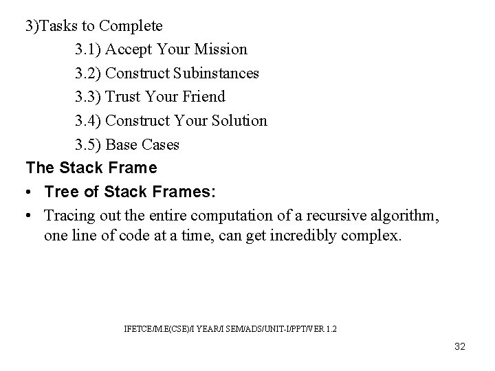
3)Tasks to Complete 3. 1) Accept Your Mission 3. 2) Construct Subinstances 3. 3) Trust Your Friend 3. 4) Construct Your Solution 3. 5) Base Cases The Stack Frame • Tree of Stack Frames: • Tracing out the entire computation of a recursive algorithm, one line of code at a time, can get incredibly complex. IFETCE/M. E(CSE)/I YEAR/I SEM/ADS/UNIT-I/PPT/VER 1. 2 32

• This is why the friends level of abstraction, which considers one stack frame at a time, is the best way to understand, explain, and design a recursive algorithm • However, it is also useful to have some picture of the entire computation. • For this, the tree-of-stack-frames level of abstraction is best. • The key thing to understand is the difference between a particular routine and a particular execution of a routine on a particular input instance. IFETCE/M. E(CSE)/I YEAR/I SEM/ADS/UNIT-I/PPT/VER 1. 2 33

• A single routine can at one moment in time have many executions going on. Each such execution is referred to as a stack frame. Stack of Stack Frames: • The algorithm is actually implemented on a computer by a stack of stack frames. What is stored in the computer memory at any given point in time is only a single path down the tree. • The tree represents what occurs throughout time. IFETCE/M. E(CSE)/I YEAR/I SEM/ADS/UNIT-I/PPT/VER 1. 2 34

Using a Stack Frame: • Recall that a stack is a data structure in which either a new element is pushed onto the top or the last element to have been added is popped off • Let us denote the top stack frame by A. When the execution of A makes a subroutine call to a routine with some input values, a stack frame is created for this new instance. • This frame denoted B is pushed onto the stack after that for A. IFETCE/M. E(CSE)/I YEAR/I SEM/ADS/UNIT-I/PPT/VER 1. 2 35

• In addition to a separate copy of the local variables for the routine, it contains a pointer to the next line of code that A must execute when B returns. • When B returns, its stack frame is popped, and A continues to execute at the line of code that had been indicated within B. • When A completes, it too is popped off the stack. IFETCE/M. E(CSE) /I YEAR/I SEM/ADS/UNIT-I/PPT/VER 1. 2 36

Proving Correctness with Strong Induction: • Strong induction is similar to induction, except that instead of assuming only S(n − 1) to prove S(n), you must assume all of S(0), S(1), S(2), . . . , S(n − 1). A Statement for Each n: For each value of n ≥ 0, let S(n) represent a Boolean statement. For some values of n this statement may be true, and for others it may be false. IFETCE/M. E(CSE)/I YEAR/I SEM/ADS/UNIT-I/PPT/VER 1. 2 37

Goal: Our goal is to prove that it is true for every value of n, namely that ∀n ≥ 0, S(n). Proof Outline: Proof by strong induction on n. Induction Hypothesis: For each n ≥ 0, let S(n) be the statement that. . (It is important to state this clearly. ) Base Case: Prove that the statement S(0) is true. Induction Step: For each n ≥ 0, prove S(0), S(1), S(2), . . . , S(n − 1) ⇒ S(n). Conclusion: By way of induction, we can conclude that ∀n ≥ 0, S(n). IFETCE/M. E(CSE)/I YEAR/I SEM/ADS/UNIT-I/PPT/VER 1. 2 38

Examples of Recursive Algorithms Sorting and Selecting Algorithms: • The classic divide-and-conquer algorithms are merge sort and quick sort. They bothhave the following basic structure. General Recursive Sorting Algorithm: • Take the given list of objects to be sorted (numbers, strings, student records, etc. ). • Split the list into two sublists. IFETCE/M. E(CSE)/I YEAR/I SEM/ADS/UNIT-I/PPT/VER 1. 2 39

• Recursively have friends sort each of the two sublists. • Combine the two sorted sublists into one entirely sorted list. • This process leads to four different algorithms, depending on the following factors, • Sizes • Work Operations on Integers: • Raising an integer to a power b. N, multiplying x × y, and matrix multiplication each have surprising divide-and-conquer algorithms. IFETCE/M. E(CSE)/I YEAR/I SEM/ADS/UNIT-I/PPT/VER 1. 2 40

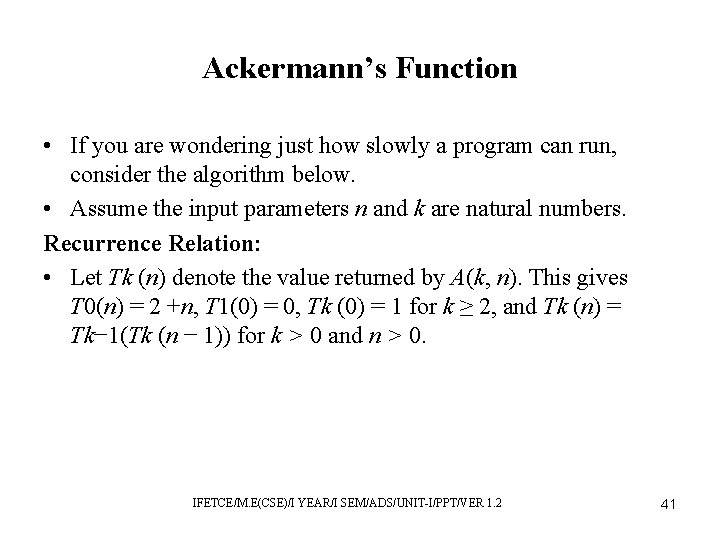
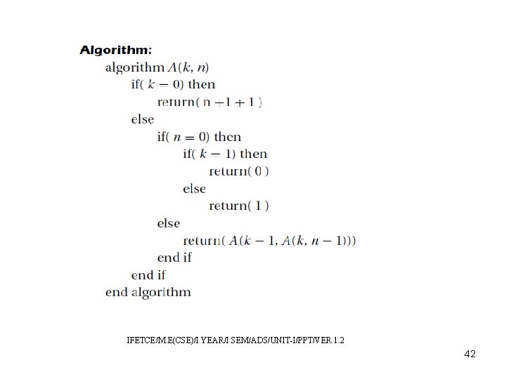
Ackermann’s Function • If you are wondering just how slowly a program can run, consider the algorithm below. • Assume the input parameters n and k are natural numbers. Recurrence Relation: • Let Tk (n) denote the value returned by A(k, n). This gives T 0(n) = 2 +n, T 1(0) = 0, Tk (0) = 1 for k ≥ 2, and Tk (n) = Tk− 1(Tk (n − 1)) for k > 0 and n > 0. IFETCE/M. E(CSE)/I YEAR/I SEM/ADS/UNIT-I/PPT/VER 1. 2 41

IFETCE/M. E(CSE)/I YEAR/I SEM/ADS/UNIT-I/PPT/VER 1. 2 42

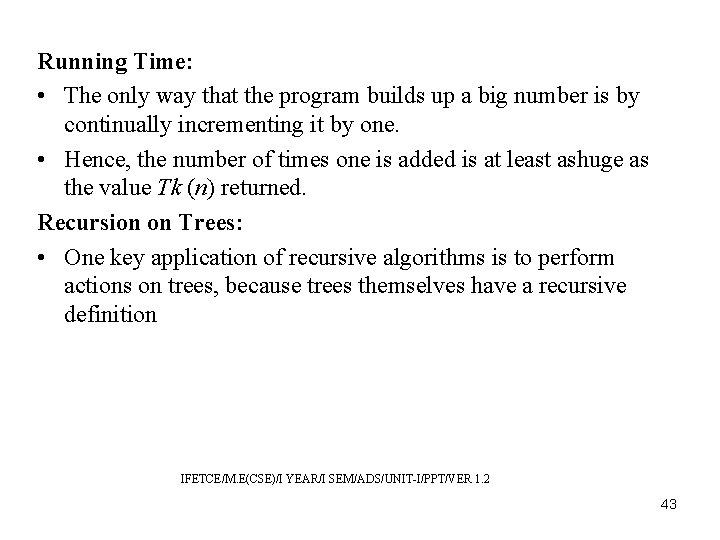
Running Time: • The only way that the program builds up a big number is by continually incrementing it by one. • Hence, the number of times one is added is at least ashuge as the value Tk (n) returned. Recursion on Trees: • One key application of recursive algorithms is to perform actions on trees, because trees themselves have a recursive definition IFETCE/M. E(CSE)/I YEAR/I SEM/ADS/UNIT-I/PPT/VER 1. 2 43

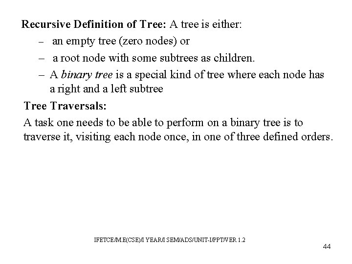
Recursive Definition of Tree: A tree is either: – an empty tree (zero nodes) or – a root node with some subtrees as children. – A binary tree is a special kind of tree where each node has a right and a left subtree Traversals: A task one needs to be able to perform on a binary tree is to traverse it, visiting each node once, in one of three defined orders. IFETCE/M. E(CSE)/I YEAR/I SEM/ADS/UNIT-I/PPT/VER 1. 2 44

• Before one becomes familiar with recursive programs, one tends to think about computation iteratively, “I visit this node first, then this one, and so on. ” • Each iteration, the program says “I just visited this node, so now let me find the next node to visit. ” Surprisingly, such a computation is hard to code. • The reason is that binary trees by their very nature have a recursive structure. IFETCE/M. E(CSE)/I YEAR/I SEM/ADS/UNIT-I/PPT/VER 1. 2 45

Examples • • • Here is a list of problems involving binary trees. 1. Return the maximum of data fields of nodes. 2. Return the height of the tree. 3. Return the number of leaves in the tree. (A harder one. ) 4. Copy the tree. IFETCE/M. E(CSE)/I YEAR/I SEM/ADS/UNIT-I/PPT/VER 1. 2 46

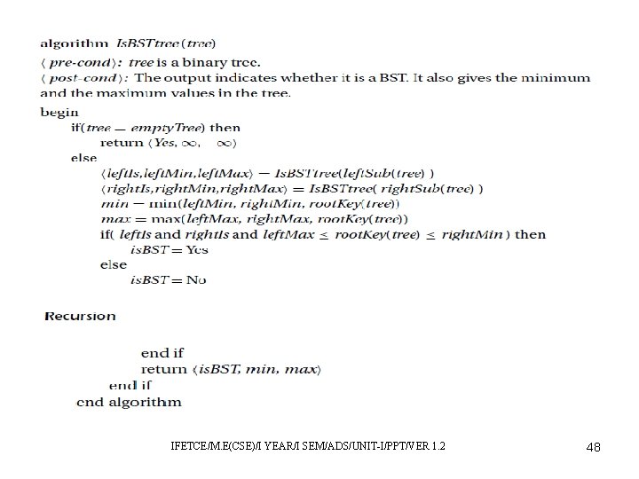
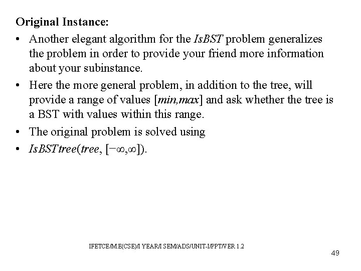
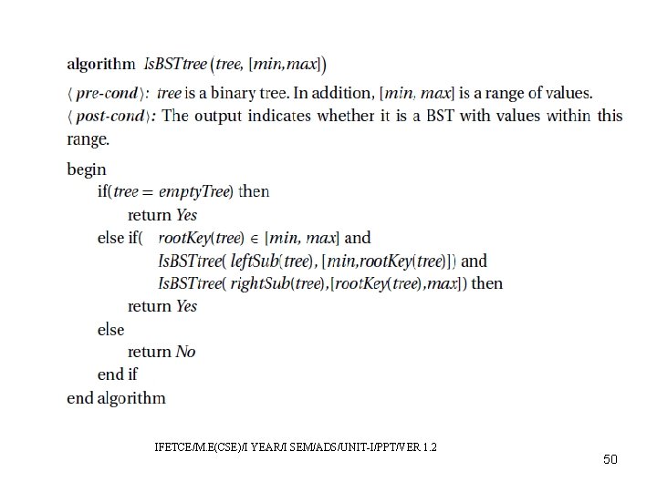
Generalizing the Problem • When writing a recursive algorithm for a problem it is easier to solve a more general version of the problem, providing more information about the original instance or asking for more information about subinstances. Subinstance: • It is better to combine the Is. BSTtree and the Min and Max routines into one routine so that the tree only needs to be traversed once. IFETCE/M. E(CSE)/I YEAR/I SEM/ADS/UNIT-I/PPT/VER 1. 2 47

IFETCE/M. E(CSE)/I YEAR/I SEM/ADS/UNIT-I/PPT/VER 1. 2 48

Original Instance: • Another elegant algorithm for the Is. BST problem generalizes the problem in order to provide your friend more information about your subinstance. • Here the more general problem, in addition to the tree, will provide a range of values [min, max] and ask whether the tree is a BST with values within this range. • The original problem is solved using • Is. BSTtree(tree, [−∞, ∞]). IFETCE/M. E(CSE)/I YEAR/I SEM/ADS/UNIT-I/PPT/VER 1. 2 49

IFETCE/M. E(CSE)/I YEAR/I SEM/ADS/UNIT-I/PPT/VER 1. 2 50

Heap Sort and Priority Queues • Heap sort is a fast sorting algorithm that is easy to implement. • Like quick sort, it has the advantage of being done in place in memory, whereas merge and radix–counting sorts require an auxiliary array of memory to transfer the data to. Completely Balanced Binary Tree: • The values being sorted as stored in a binary tree that is completely balanced, i. e. , every level of the tree is completely full except for the bottom level, which is filled in fromthe left. IFETCE/M. E(CSE)/I YEAR/I SEM/ADS/UNIT-I/PPT/VER 1. 2 51

Definition of a Heap: • A heap imposes a partial order on the set of values, requiring that the value of each node be greater than or equal to that of each of the node’s children. • There are no rules about whether the left or the right child is larger. Maximum at Root: • An implication of the heap rules is that the root contains the maximum value. • The maximum may appear repeatedly in other places as well. IFETCE/M. E(CSE)/I YEAR/I SEM/ADS/UNIT-I/PPT/VER 1. 2 52

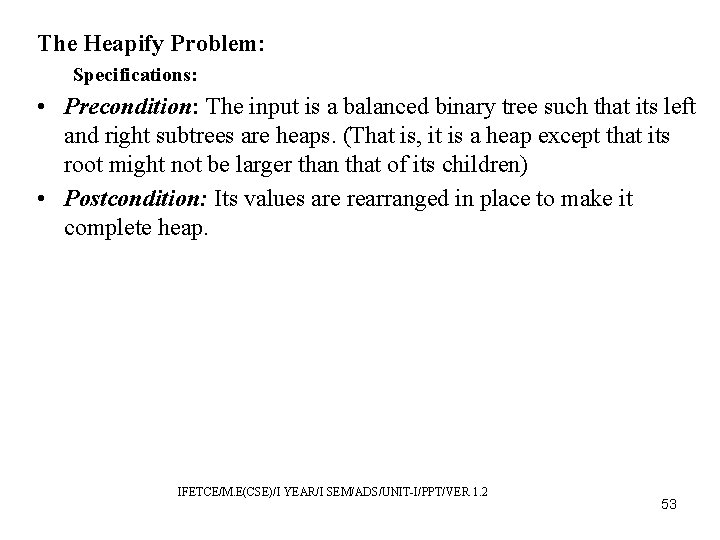
The Heapify Problem: Specifications: • Precondition: The input is a balanced binary tree such that its left and right subtrees are heaps. (That is, it is a heap except that its root might not be larger than that of its children) • Postcondition: Its values are rearranged in place to make it complete heap. IFETCE/M. E(CSE)/I YEAR/I SEM/ADS/UNIT-I/PPT/VER 1. 2 53

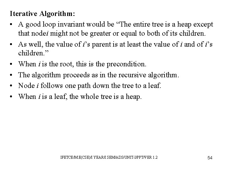
Iterative Algorithm: • A good loop invariant would be “The entire tree is a heap except that nodei might not be greater or equal to both of its children. • As well, the value of i’s parent is at least the value of i and of i’s children. ” • When i is the root, this is the precondition. • The algorithm proceeds as in the recursive algorithm. • Node i follows one path down the tree to a leaf. • When i is a leaf, the whole tree is a heap. IFETCE/M. E(CSE)/I YEAR/I SEM/ADS/UNIT-I/PPT/VER 1. 2 54

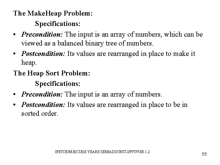
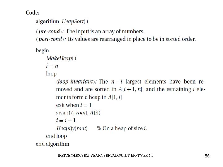
The Make. Heap Problem: Specifications: • Precondition: The input is an array of numbers, which can be viewed as a balanced binary tree of numbers. • Postcondition: Its values are rearranged in place to make it heap. The Heap Sort Problem: Specifications: • Precondition: The input is an array of numbers. • Postcondition: Its values are rearranged in place to be in sorted order. IFETCE/M. E(CSE)/I YEAR/I SEM/ADS/UNIT-I/PPT/VER 1. 2 55

IFETCE/M. E(CSE)/I YEAR/I SEM/ADS/UNIT-I/PPT/VER 1. 2 56

Priority Queues • Like stacks and queues, priority queues are an important ADT. • Definition: A priority queue consists of: – Data: A set of elements, each of which is associated with an integer that is referred to as the priority of the element. IFETCE/M. E(CSE)/I YEAR/I SEM/ADS/UNIT-I/PPT/VER 1. 2 57

Operations: Insert an Element: An element, along with its priority, is added to the queue. Change Priority: The priority of an element already in the queue is changed. The routine is passed a pointer to the element within the priority queue and its new priority. Remove an Element: Removes and returns an element of the highest priority fromthe queue. IFETCE/M. E(CSE)/I YEAR/I SEM/ADS/UNIT-I/PPT/VER 1. 2 58

Representing Expressions with Trees • consider how to represent multivariate expressions using binary trees. • We will develop the algorithms to evaluate, copy, differentiate, simplify, and print such an expression. • Though these are seemingly complex problems, they have simplerecursive solutions. IFETCE/M. E(CSE)/I YEAR/I SEM/ADS/UNIT-I/PPT/VER 1. 2 59

Recursive Definition of an Expression: • Single variables x, y, and z and single real values are themselves expressions. • If f and g are expressions, then f + g, f − g, f ∗ g, and f/g are also expressions. Tree Data Structure: The recursive definition of an expression directly mirrors that of a binary tree. Because of this, a binary tree is a natural data structure for storing an expression. (Conversely, you can use an expression to represent a binary tree. ) IFETCE/M. E(CSE)/I YEAR/I SEM/ADS/UNIT-I/PPT/VER 1. 2 60