Unit 9 Sampling Unit 8 theory Unit 9

Unit 9: Sampling

Unit 8: theory, Unit 9 (et seq): practice • In Unit 8, we knew the distribution (µ, σ) of the box (population) – found probable values for sample’s x, s (i. e. , EV and SE of avg) • In Unit 9, we take a sample, find its x, s – use them to estimate population’s µ, σ

How close is your poll? (I) • Ex: Poll of 1600 people: 1120 are against NYRI (New York Regional Interconnect proposes building a power line from just north of here to NYC suburbs). – Best guess for % in area who are against it? 1120/1600 = 70%. (What else? ) – How far off might this guess be? I’m “ 68% confident” that it will be within one SE for %, √[. 7 • . 3]/√ 1600 = 1. 1% , of right answer. • std error for % = σ/√n = √[p(1 -p)] / √n • “bootstrapping”: this p is the sample %; we don’t know the population %, so √[p(1 -p)] is the best guess we can make for σ.

Normal table z Area(%) z Area(%) 0. 0 0. 9 63. 19 1. 8 92. 81 2. 7 99. 31 3. 6 99. 968 0. 05 3. 99 0. 95 65. 79 1. 85 93. 57 2. 75 99. 4 3. 65 99. 974 0. 1 7. 97 1 68. 27 1. 9 94. 26 2. 8 99. 49 3. 7 99. 978 0. 15 11. 92 1. 05 70. 63 1. 95 94. 88 2. 85 99. 56 3. 75 99. 982 0. 2 15. 85 1. 1 72. 87 2 95. 45 2. 9 99. 63 3. 8 99. 986 0. 25 19. 74 1. 15 74. 99 2. 05 95. 96 2. 95 99. 68 3. 85 99. 988 0. 3 23. 58 1. 2 76. 99 2. 1 96. 43 3 99. 73 3. 9 99. 99 0. 35 27. 37 1. 25 78. 87 2. 15 96. 84 3. 05 99. 771 3. 95 99. 992 0. 4 31. 08 1. 3 80. 64 2. 2 97. 22 3. 1 99. 806 4 99. 9937 0. 45 34. 73 1. 35 82. 3 2. 25 97. 56 3. 15 99. 837 4. 05 99. 9949 0. 5 38. 29 1. 4 83. 85 2. 3 97. 86 3. 2 99. 863 4. 1 99. 9959 0. 55 41. 77 1. 45 85. 29 2. 35 98. 12 3. 25 99. 885 4. 15 99. 9967 0. 6 45. 15 1. 5 86. 64 2. 4 98. 36 3. 3 99. 903 4. 2 99. 9973 0. 65 48. 43 1. 55 87. 89 2. 45 98. 57 3. 35 99. 919 4. 25 99. 9979 0. 7 51. 61 1. 6 89. 04 2. 5 98. 76 3. 4 99. 933 4. 3 99. 9983 0. 75 54. 67 1. 65 90. 11 2. 55 98. 92 3. 45 99. 944 4. 35 99. 9986 0. 8 57. 63 1. 7 91. 09 2. 6 99. 07 3. 5 99. 953 4. 4 99. 9989 0. 85 60. 47 1. 75 91. 99 2. 65 99. 2 3. 55 99. 961 4. 45 99. 9991

How close is your poll? (II) • Ex: Poll of 1600 people says 1120 are against NYRI. – Best guess for % in area who are against it? 70%. – “ 95% confidence interval” for population %: 70% ± (2 • (std error) = 2. 2%) • 67. 8% to 72. 2% – 98% CI: 70% ± (2. 35 • (std error)= 2. 7%) • 67. 3% to 72. 7%

Odd ex: Know population, guess sample! The 10 million people in a state own an avg of 10 shirts (or blouses, or tops, or. . . ), with an SD of 4, but 3 million own at least 12. In a simple random sample of 1600: (a)What is the probability that the avg # of shirts of people in sample is at least 12? (b)What is the probability that at least 500 people in sample own at least 12 shirts? (a) Box values are numbers of shirts. EV of avg = 10, SE of avg = 4/√ 1600 =. 1, so 12 in std units is z = (12 -10)/. 1 = 20, and P(z ≥ 20) is negligible. (b) Box is 30% 1’s, 70% 0’s. EV of count = 1600(. 3) = 480, SE = √[(. 3)(. 7)]√ 1600 ≈ 18. 3. P(count ≥ 500) = P(z ≥ (500480)/18. 3 ≈ 1. 09) ≈ ((100 -72)/2)% = 14%.

Small population, big sample? In surveying, we usually look for a “simple random sample” – don’t interview the same person twice. But that means drawing from the “box” without replacement, and our theory assumed with replacement. What changes? : SE of avg (or %) w/o repl = (SE of avg with repl)∙(“correction factor”) “cf” = √[(# in pop - # in sample)/(# in pop - 1)] So unless pop is small & sample is a big fraction of it, we can ignore the cf.

(Rare) example that might need cf Of 2500 Purdue faculty, ask 100 their choice for faculty president. 40 say Abhyankar. What is a 95% CI for % of whole faculty for Abhyankar? cf = √[(2500 - 100)/(2500 - 1)] ≈. 98 (close to 1, even though 100 is 4% of whole faculty), so requested CI is 40% ± 2(. 98)√(. 4)(. 6)/√ 100 = 40% ± 9. 6% (not very accurate, despite polling 4%).

More examples • A poll of 2000 NY citizens show 1246 of them prefer chocolate to vanilla. What is a 95% CI for the % of all NYers who prefer chocolate? – (How about an 80% CI? ) • A poll of 200 Colgate students show 2 of them believe in the Easter Bunny. What is a 95% CI for the % of all CU students who believe in EB? – Don’t trust CI if it includes values >100% or <0%

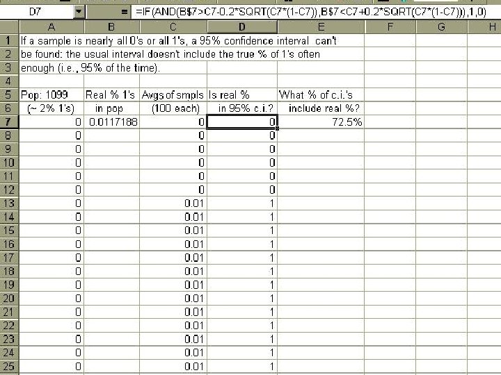
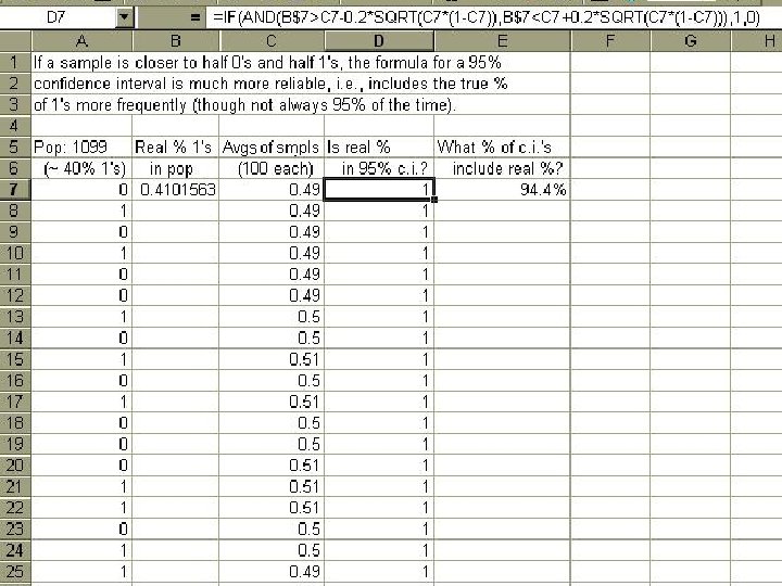
When the fraction p of a 0 -1 distribution is close to 0% or 100%, the standard deviation σ , given by √[p(1 -p)] , is small; but this effect becomes noticeable only very close to 0% or 100%. In particular, σ is at least half its maximum value of. 5 except for p < 7% or p > 93%.

Guess µ of numerical variable (not %) • What changes? – (bootstrap) std error = s / √n • (i. e. approximate pop SD by sample SD • . . . because when the box isn’t 1 -0, the avg doesn’t give the SD) – if n is small (rare in surveys, more common in lab studies), use t-table instead of z-table • Which row in t-table depends on n-1 (df) • Recall s = SD+ = σ ∙√[n/(n-1)] > σ • (For n > 25, t-table is indistinguishable from z-table and formula for s is very close to formula for σ )

Example: CI for num variable 20 students take an exam (cold), avg score 72, s = 10. What’s a 95% CI for avg score of all students on that exam? – 72 ± 2. 09(10/√ 20) = 72 ± 4. 7 Remember: This is a 95% CI for the avg of all students. Interval to be 95% sure of including score of any particular student is still 72 ± 2(10).

More examples • A random sample of 900 have avg income $32, 000, with an SD of $15, 000. What should we guess is the avg income of the population from which we drew, give or take how much? • A random sample of 400 people has avg age 40, with an SD of 25. What should we guess is the population’s avg age, give or take how much? • A market survey of 100 households says 10% use Excrud for dishes. What % of the country uses Excrud, give or take how much?

How large a sample needed? (I) • For %, estimate p and solve for n: – n = z 2 p(1 -p) / tolerance 2 – Ex: How many people should we survey to get % of voters in favor of Smith within 2% (95% CI)? Probably about 20% favor Smith. • … or just note p(1 -p) ≤ 0. 25:

How large a sample needed? (II) • For estimates of µ, must guess σ – (because we can’t get σ from µ ) – Again, solve for n : z 2 σ2 / tolerance 2 • Ex: To estimate within 2 pts (95% CI) the population’s avg score on an exam, how big a sample is needed? Guess σ = 10. – [Answer: 96. ]

Sample size needed doesn’t depend on population! The sample size computations we just did don’t involve the size of the population (as long as it’s reasonably large). To get the same accuracy, we need the sample size in Utica, Phoenix or Tokyo. As the text says, the Texan is wrong!