UNIT 5 Classification Prediction and Cluster analysis What

UNIT – 5 Classification , Prediction and Cluster analysis

What is Classification and Prediction? Ø Classification and prediction are two forms of data analysis that can be used to extract models describing important data classes or to predict future data trends. Ø Such analysis can help provide us with a better understanding of the data at large. Whereas § classification predicts categorical (discrete, unordered) labels, § prediction models continuous valued functions. Ø For example, § we can build a classification model to categorize bank loan applications as either safe or risky § A prediction model to predict the expenditures in dollars of potential customers on computer equipment given their income and occupation. Ø Applications of Classification and Predication: Credit approval, Target marketing, Medical diagnosis, Fraud detection Ø Recent data mining research has built on such work, developing scalable classification and prediction techniques capable of handling large disk-resident data.

How does classification work? Ø Data classification is a two-step process Ø Model construction: describing a set of predetermined classes § Each tuple/sample is assumed to belong to a predefined class, as determined by the class label attribute § The set of tuples used for model construction is training set. § The model is represented as classification rules, decision trees, or mathematical formula. Ø Model usage: for classifying future or unknown objects § Estimate accuracy of the model § § § The known label of test sample is compared with the classified result from the model Accuracy rate is the percentage of test set samples that are correctly classified by the model If the accuracy is acceptable, use the model to classify data tuples whose class labels are not known

Step 1: Model Construction Learning: Training data are analyzed by a classification algorithm. Here, the class label attribute is loan decision, and the learned model or classifier is represented in the form of classification rules.

Step 2: Using the Model in Prediction Classification: Test data are used to estimate the accuracy of the classification rules. If the accuracy is considered acceptable, the rules can be applied to the classification of new data tuples.

Issues regarding classification and prediction

Issues: Data Preparation Ø Data cleaning § This refers to the preprocessing of data in order to remove or reduce noise (by applying smoothing techniques) and the treatment of missing values (e. g. , by replacing a missing value with the most commonly occurring value for that attribute, or with the most probable value based on statistics). Ø Relevance analysis (feature selection) § Remove the redundant data from the database using the Correlation or other statistical method. § Remove the irrelevant attributes from the database using Attribute subset selection method. Ø Data transformation § The data may be transformed by normalization, particularly when neural networks or methods involving distance measurements are used in the learning step. § The data can also be transformed by generalizing it to higher-level concepts. This is particularly useful for continuous valued attributes. For example, numeric values for the attribute income can be generalized to discrete ranges, such as low, medium, and high.

Issues: Evaluating Classification Methods Ø Accuracy: § The accuracy of a classifier refers to the ability of a given classifier to correctly predict the class label of new or previously unseen data. § Similarly, the accuracy of a predictor refers to how well a given predictor can guess the value of the predicted attribute for new or previously unseen data. Ø Speed: This refers to the computational costs involved in generating and using the given classifier or predictor. Ø Robustness: This is the ability of the classifier or predictor to make correct predictions given noisy data or data with missing values. Ø Scalability: This refers to the ability to construct the classifier or predictor efficiently given large amounts of data. Ø Interpretability: This refers to the level of understanding and insight that is provided by the classifier or predictor. Interpretability is subjective and therefore more difficult to assess. Ø Other measures, e. g. , goodness of rules, such as decision tree size or compactness of classification rules

Classification by decision tree induction

Classification by decision tree induction Decision tree induction is the learning of decision trees from class-labeled training tuples. A decision tree is a flowchart-like tree structure, where each internal node denotes a test on an attribute, each branch represents an outcome of the test, and each leaf node holds a class label. The topmost node in a tree is the root node. § A decision tree for the concept buys computer, indicating whether a customer at All. Electronics is likely to purchase a computer. § Each internal (nonleaf) node represents a test on an attribute. § Each leaf node represents a class (either buys computer = yes or buys computer = no).

Classification by decision tree induction How are decision trees used for classification? Given a tuple, X, for which the associated class label is unknown, the attribute values of the tuple are tested against the decision tree. A path is traced from the root to a leaf node, which holds the class prediction for that tuple. Decision trees can easily be converted to classification rules. Why are decision tree classifiers so popular? § The construction of decision tree classifiers does not require any domain knowledge or parameter setting, and therefore is appropriate for exploratory knowledge discovery. § Decision trees can handle high dimensional data. § Their representation of acquired knowledge in tree form is easy to understand by humans. § The learning and classification steps of decision tree induction are simple and fast. § In general, decision tree classifiers have good accuracy. However, successful use may depend on the data at hand. Decision tree induction algorithms have been used for classification in many application areas, such as medicine, manufacturing and production, financial analysis, astronomy, and molecular biology.

Algorithm for decision tree induction Ø Basic algorithm (a greedy algorithm) § Tree is constructed in a top-down recursive divide-and-conquer manner § At start, all the training examples are at the root § Attributes are categorical (if continuous-valued, they are discretized in advance) § Examples are partitioned recursively based on selected attributes § Test attributes are selected on the basis of a heuristic or statistical measure (e. g. , information gain) Ø Conditions for stopping partitioning § All samples for a given node belong to the same class § There are no remaining attributes for further partitioning – majority voting is employed for classifying the leaf § There are no samples left Generate a decision tree from the training tuples of data partition D. Data partition D, which is a set of training tuples and their associated class labels; Attribute list, the set of candidate attributes; Attribute selection method, a procedure to determine the splitting criterion that “best” partitions the data tuples into individual classes. This criterion consists of a splitting attribute and, possibly, either a split point or splitting subset.

Algorithm for decision tree induction (1) create a node N; (2) if tuples in D are all of the same class, C then (3) return N as a leaf node labeled with the class C; (4) if attribute list is empty then (5) return N as a leaf node labeled with the majority class in D; // majority voting (6) apply Attribute selection method(D, attribute list) to find the “best” splitting criterion; (7) label node N with splitting criterion; (8) if splitting attribute is discrete-valued and multiway splits allowed then (9) attribute list = attribute list - splitting attribute; // remove splitting attribute (10) for each outcome j of splitting criterion // partition the tuples and grow subtrees for each partition (11) let Dj be the set of data tuples in D satisfying outcome j; // a partition (12) if Dj is empty then (13) attach a leaf labeled with the majority class in D to node N; (14) else attach the node returned by Generate decision tree(Dj, attribute list) to node N; endfor (15) return N;

Partitioning Scenarios Three possibilities for partitioning tuples based on the splitting criterion, shown with examples. Let A be the splitting attribute. (a) If A is discrete-valued, then one branch is grown for each known value of A. (b) If A is continuous-valued, then two branches are grown, corresponding to A split point and A > split point. (c) If A is discrete-valued and a binary tree must be produced, then the test is of the form A ϵ SA, where SA is the splitting subset for A. a b c

Attribute Selection Measure: Information Gain (ID 3) Ø Select the attribute with the highest information gain Ø Let pi be the probability that an arbitrary tuple in D belongs to class Ci, estimated by |Ci, D|/|D| Ø Expected information (entropy) needed to classify a tuple in D: Ø Information needed (after using A to split D into v partitions) to classify D: Ø Information gained by branching on attribute A

Attribute Selection Measure: Information Gain (ID 3) Class P: buys_computer = “yes” g Class N: buys_computer = “no” g means “age <=30” has 5 out of 14 samples, with 2 yes’es and 3 no’s.

Computing Information-Gain for Continuous-Valued Attributes Ø Let attribute A be a continuous-valued attribute Ø Must determine the best split point for A § Sort the value A in increasing order § Typically, the midpoint between each pair of adjacent values is considered as a possible split point § (ai+ai+1)/2 is the midpoint between the values of ai and ai+1 § The point with the minimum expected information requirement for A is selected as the split-point for A Ø Split: D 1 is the set of tuples in D satisfying A ≤ split-point, and D 2 is the set of tuples in D satisfying A > split-point

Comparing Attribute Selection Measures • The three measures, in general, return good results but – Information gain (ID 3): • biased towards multi valued attributes – Gain ratio (C 4. 5): • tends to prefer unbalanced splits in which one partition is much smaller than the others – Gini index (CART): • biased to multi valued attributes • has difficulty when # of classes is large • tends to favor tests that result in equal-sized partitions and purity in both partitions

Overfitting and Tree Pruning § When a decision tree is built, many of the branches will reflect anomalies in the training data due to noise or outliers. § Tree pruning methods address this problem of overfitting the data. Such methods typically use statistical measures to remove the least reliable branches. § Pruned trees tend to be smaller and less complex and, thus, easier to comprehend. § They are usually faster and better at correctly classifying independent test data (i. e. , of previously unseen tuples) than unpruned trees. Two approaches to avoid overfitting Prepruning: Halt tree construction early by deciding not to further split or partition the subset of training tuples at a given node. Upon halting, the node becomes a leaf. Difficult to choose an appropriate threshold Postpruning: Remove branches from a “fully grown”. A subtree at a given node is pruned by removing its branches and replacing it with a leaf. The leaf is labeled with the most frequent class among the subtree being replaced.

In example, notice the subtree at node “A 3? ” in the unpruned tree of Figure Suppose that the most common class within this subtree is “class B. ” In the pruned version of the tree, the subtree in question is pruned by replacing it with the leaf “class B. ”

Bayesian classification

What are Bayesian classifiers? Ø Bayesian classifiers are statistical classifiers. Ø They can predict class membership probabilities, such as the probability that a given tuple belongs to a particular class. Ø Bayesian classification is based on Bayes’ theorem. Ø Studies comparing classification algorithms have found a simple Bayesian classifier known as the naïve Bayesian classifier to be comparable in performance with decision tree. Ø Performance: Bayesian classifiers have also exhibited high accuracy and speed when applied to large databases. Ø Incremental: Each training example can incrementally increase/decrease the probability that a hypothesis is correct. prior knowledge can be combined with observed data Ø Standard: Even when Bayesian methods are computationally intractable, they can provide a standard of optimal decision making against which other methods can be measured.

What are Bayesian classifiers? Ø Bayes’ theorem is named from Thomas Bayes, who did early work in probability and decision theory during the 18 th century Ø Let X be a data sample (“evidence”): class label is unknown Ø Let H be a hypothesis that X belongs to class C Ø Classification is to determine P(H|X), the posteriori probability of the hypothesis based on the observed data sample X. In other words, we are looking for the probability that tuple X belongs to class C, given that we know the attribute description of X. Ø For example, suppose our world of data tuples is confined to customers described by the attributes age and income, respectively, and that X is a 35 -year-old customer with an income of $40, 000. Suppose that H is the hypothesis that our customer will buy a computer. Then P(H|X) reflects the probability that customer X will buy a computer given that we know the customer’s age and income.

Bayesian classifiers Cont… Ø In contrast, P(H) is the prior probability of H. For our example, this is the probability that any given customer will buy a computer, regardless of age, income, or any other information, for that matter. Ø The prior probability P(H), which is independent of X. Ø Similarly, P(X|H) is the posterior probability of X conditioned on H. That is, it is the probability that a customer, X, is 35 years old and earns $40, 000, given that we know the customer will buy a computer. Ø P(X) is the prior probability of X. Using our example, it is the probability that a person from our set of customers is 35 years old and earns $40, 000. Ø Given training data X, posteriori probability of a hypothesis H, P(H|X), follows the Bayes’ theorem Ø Informally, this can be written as posteriori = likelihood x prior/evidence

Towards Naïve Bayesian Classifier Ø Let D be a training set of tuples and their associated class labels (table cell value), and each tuple is represented by an n-D attribute (table fields) vector X = (x 1, x 2, …, xn) Ø Suppose there are m classes C 1, C 2, …, Cm. For example (buy_computer=“YES”, buy_computer=“NO”) Ø Classification is to derive the maximum posteriori, i. e. , the maximal P(Ci|X) Ø This can be derived from Bayes’ theorem Ø Since P(X) is constant for all classes, only needs to be maximized

Towards Naïve Bayesian Classifier Ø Given data sets with many attributes, it would be extremely computationally expensive to compute P(X|Ci). Ø In order to reduce computation in evaluating P(X|Ci), the naive assumption of class conditional independence is made. Ø This presumes that the values of the attributes are conditionally independent of one another, given the class label of the tuple (i. e. , that there are no dependence relationships among the attributes). Thus, Ø We can easily estimate the probabilities P(x 1|Ci), P(x 2|Ci), , : : : , P(xn|Ci) from the training tuples.

Naïve Bayes Classifier: Training Dataset Class: C 1: buys_computer = ‘yes’ C 2: buys_computer = ‘no’ Data to be classified: X = (age <=30, Income = medium, Student = yes Credit_rating = Fair)

Naïve Bayes Classifier: An Example • P(Ci): P(buys_computer = “yes”) = 9/14 = 0. 643 P(buys_computer = “no”) = 5/14= 0. 357 • Compute P(X|Ci) for each class P(age = “<=30” | buys_computer = “yes”) = 2/9 = 0. 222 P(age = “<= 30” | buys_computer = “no”) = 3/5 = 0. 6 P(income = “medium” | buys_computer = “yes”) = 4/9 = 0. 444 P(income = “medium” | buys_computer = “no”) = 2/5 = 0. 4 P(student = “yes” | buys_computer = “yes) = 6/9 = 0. 667 P(student = “yes” | buys_computer = “no”) = 1/5 = 0. 2 P(credit_rating = “fair” | buys_computer = “yes”) = 6/9 = 0. 667 P(credit_rating = “fair” | buys_computer = “no”) = 2/5 = 0. 4 • X = (age <= 30 , income = medium, student = yes, credit_rating = fair) P(X|Ci) : P(X|buys_computer = “yes”) = 0. 222 x 0. 444 x 0. 667 = 0. 044 P(X|buys_computer = “no”) = 0. 6 x 0. 4 x 0. 2 x 0. 4 = 0. 019 P(X|Ci)*P(Ci) : P(X|buys_computer = “yes”) * P(buys_computer = “yes”) = 0. 028 P(X|buys_computer = “no”) * P(buys_computer = “no”) = 0. 007 Therefore, X belongs to class (“buys_computer = yes”)

Avoiding the Zero-Probability Problem Ø Naïve Bayesian prediction requires each conditional prob. be non-zero. Otherwise, the predicted prob. will be zero Ø Ex. Suppose a dataset with 1000 tuples, income=low (0), income= medium (990), and income = high (10) Ø Use Laplacian correction (or Laplacian estimator) – Adding 1 to each case Prob(income = low) = 1/1003 Prob(income = medium) = 991/1003 Prob(income = high) = 11/1003 – The “corrected” prob. estimates are close to their “uncorrected” counterparts

Naïve Bayes Classifier: Comments • Advantages – Easy to implement – Good results obtained in most of the cases • Disadvantages – Assumption: class conditional independence, therefore loss of accuracy – Practically, dependencies exist among variables • E. g. , hospitals: patients: Profile: age, family history, etc. Symptoms: fever, cough etc. , Disease: lung cancer, diabetes, etc. • Dependencies among these cannot be modeled by Naïve Bayes Classifier • How to deal with these dependencies? Bayesian Belief Networks

Rule – Based Classification

Using IF-THEN Rules for Classification Ø Rules are a good way of representing information or bits of knowledge. A rule-based classifier uses a set of IF-THEN rules for classification. Ø An IF-THEN rule is an expression of the form IF condition THEN conclusion. An example is rule R 1, R 1: IF age = youth AND student = yes THEN buys computer = yes. R 1 can also be written as R 1: (age = youth) ^ (student = yes)) (buys computer = yes). Ø The “IF”-part (or left-hand side)of a rule is known as the rule antecedent or precondition. Ø The “THEN”-part (or right-hand side) is the rule consequent. Ø In the rule antecedent, the condition consists of one or more attribute tests (such as age = youth, and student = yes) that are logically ANDed. Ø The rule’s consequent contains a class prediction.

Using IF-THEN Rules for Classification Ø A rule R can be assessed by its coverage and accuracy. Given a tuple X, from a class labeled data set D, § let ncovers be the number of tuples covered by R; § ncorrect be the number of tuples correctly classified by R; § |D| be the number of tuples in D. Ø We can define the coverage and accuracy of R as § coverage(R) = ncovers / |D| § accuracy(R) = ncorrect / ncovers Ø That is, a rule’s coverage is the percentage of tuples that are covered by the rule. Ø For a rule’s accuracy, we look at the tuples that it covers and see what percentage of them the rule can correctly classify. Ø For Example: Consider rule R 1, which covers 2 of the 14 tuples. It can correctly classify both tuples. Ø Therefore, coverage(R 1) = 2/14 = 14: 28% and accuracy (R 1) = 2/2 = 100%.

Using IF-THEN Rules for Classification If more than one rule is triggered, we need a conflict resolution strategy to figure out which rule gets to fire and assign its class prediction to X. There are many possible strategies. 1. The size ordering scheme assigns the highest priority to the triggering rule that has the “toughest” requirements, where toughness is measured by the rule antecedent size. That is, the triggering rule with the most attribute tests is fired. 2. class-based ordering, the classes are sorted in order of decreasing “importance, ” such as most prevalent (or most frequent) class come first, the rules for the next prevalent class come next, and so on. 3. Rule-based ordering, the rules are organized into one long priority list, according to some measure of rule quality such as accuracy, coverage, or size (number of attribute tests in the rule antecedent), or based on advice from domain experts. When rule ordering is used, the rule set is known as a decision list.

Rule Extraction from a Decision Tree n Rules are easier to understand than large trees n One rule is created for each path from the root to a leaf n Each attribute-value pair along a path forms a conjunction: the leaf holds the class prediction n Rules are mutually exclusive and exhaustive Example: Rule extraction from our buys_computer decision-tree IF age = young AND student = no IF age = young AND student = yes IF age = mid-age IF age = old AND credit_rating = excellent IF age = old AND credit_rating = fair THEN buys_computer = no THEN buys_computer = yes

Rule Extraction from Training Data Ø IF-THEN rules can be extracted directly from the training data (i. e. , without having to generate a decision tree first) using a sequential covering algorithm. Ø Sequential covering algorithms are the most widely used approach to mining disjunctive sets of classification rules. Ø There are many sequential covering algorithms. Popular variations include AQ, CN 2, and RIPPER. Ø The general strategy is as follows. § Rules are learned one at a time. § Each time a rule is learned, the tuples covered by the rule are removed, § The process repeats on the remaining tuples. Ø In this way, the rules learned should be of high accuracy. The rules need not necessarily be of high coverage. Ø This sequential learning of rules is in contrast to decision tree induction.

Example of Rule Extraction from Training Data A general-to-specific search through rule space.

What is Prediction? Ø (Numerical) prediction is similar to classification § construct a model § use model to predict continuous or ordered value for a given input Ø Prediction is different from classification § Classification refers to predict categorical class label § Prediction models continuous-valued functions Ø Major method for prediction: regression § model the relationship between one or more independent or predictor variables and a dependent or response variable Ø Regression analysis § Linear and multiple regression § Non-linear regression § Other regression methods: generalized linear model, Poisson regression, log-linear models, regression trees

Regression Analysis Ø Regression analysis can be used to model the relationship between one or more independent or predictor variables and a dependent or response variable. Ø In the context of data mining, the predictor variables are the attributes of interest describing the tuple (i. e. , making up the attribute vector). Ø In general, the values of the predictor variables are known. The response variable is what we want to predict. Ø Regression analysis is a good choice when all of the predictor variables are continuous valued as well. Ø Many problems can be solved by linear regression, and even more can be tackled by applying transformations to the variables so that a nonlinear problem can be converted to a linear one

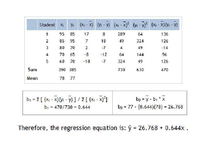
Linear Regression Ø Straight-line regression analysis involves a response variable, y, and a single predictor variable, x. Ø It is the simplest form of regression, and models y as a linear function of x. That is, y = b+wx; where the variance of y is assumed to be constant, and b and w are regression coefficients specifying the Y-intercept and slope of the line, respectively. Ø The regression coefficients, w and b, can also be thought of as weights, so that we can equivalently write, y = w 0+w 1 x Ø These coefficients can be solved for by the method of least squares, which estimates the best-fitting straight line as the one that minimizes the error between the actual data and the estimate of the line.

Linear Regression Example We model the relationship that salary may be related to the number of years of work experience with the equation y = w 0+w 1 x. Experience (x) 3 8 9 13 3 6 11 21 1 16 Salary in Thousand (y) 30 57 64 72 36 43 59 90 20 83 Aptitude Test Marks (x) 95 85 80 70 60 Statistical Grade (y) 85 95 70 65 70

Multiple Linear Regression Ø Multiple linear regression is an extension of straight-line regression so as to involve more than one predictor variable. Ø It allows response variable y to be modeled as a linear function of, say, n predictor variables or attributes, A 1, A 2, : : : , An, describing a tuple, X. (That is, X = (x 1, x 2, : : : , xn). ) Our training data set, D, contains data of the form (X 1, y 1), (X 2, y 2), : : : , (X|D|, y|D|), where the Xi are the n-dimensional training tuples with associated class labels, yi. Ø An example of a multiple linear regression model based on two predictor attributes or variables, A 1 and A 2, is y = w 0+w 1 x 1+w 2 x 2 where x 1 and x 2 are the values of attributes A 1 and A 2, respectively, in X. Ø The method of least squares shown above can be extended to solve for w 0, w 1, and w 2. Ø The equations, however, become long and are tedious to solve by hand. Multiple regression problems are instead commonly solved with the use of statistical software packages, such as SAS, SPSS, and S-Plus.

Cluster Analysis § The process of grouping a set of physical or abstract objects into classes of similar objects is called clustering. § A cluster is a collection of data objects that are similar to one another within the same cluster and are dissimilar to the objects in other clusters. § A cluster of data objects can be treated collectively as one group and so may be considered as a form of data compression. § Although classification is an effective means for distinguishing groups or classes of objects, it requires the often costly collection and labeling of a large set of training tuples or patterns, which the classifier uses to model each group. It is often more desirable to proceed in the reverse direction: First partition the set of data into groups based on data similarity (e. g. , using clustering), and then assign labels to the relatively small number of groups. § Additional advantages of such a clustering-based process are that it is adaptable to changes and helps single out useful features that distinguish different groups.

Cluster Analysis § Cluster analysis is an important human activity. Early in childhood, we learn how to distinguish between cats and dogs, or between animals and plants, by continuously improving subconscious clustering schemes. § By automated clustering, we can identify dense and sparse regions in object space and, therefore, discoverall distribution patterns and interesting correlations among data attributes. § Cluster analysis has been widely used in numerous applications, including market research, pattern recognition, data analysis, and image processing. § Clustering is also called data segmentation in some applications because clustering partitions large data sets into groups according to their similarity. § Clustering can also be used for outlier detection, where outliers (values that are “far away” from any cluster) may be more interesting than common cases. § Applications of outlier detection include the detection of credit card fraud and the monitoring of criminal activities in electronic commerce.

Types of Data in Cluster Analysis Main memory-based clustering algorithms typically operate on either of the following two data structures. Data matrix ( object-by-variable structure): § This represents n objects, such as persons, with p variables (attributes), such as age, height, weight, gender, and so on. § Two mode matrix The structure is in the form of a relational table, or n-by-p matrix (n objects p variables) Dissimilarity matrix (object-by-object structure): § This stores a collection of proximities that are available for all pairs of n objects. It is often One mode matrix represented by an n-by-n table: § where d(i, j) is the measured difference or dissimilarity between objects i and j. § In general, d(i, j) is a nonnegative number that is close to 0 when objects i and j are highly similar, and becomes larger the more they differ.

Compute Dissimilarity between Objects we discuss how object dissimilarity can be computed for objects described § by interval-scaled variables; § by binary variables; § by categorical

Interval Scaled Variables What are interval-scaled variables? Interval-scaled variables are continuous measurements of a roughly linear scale. Typical examples include weight and height and weather temperature. § Standardize data: To standardize measurements, one choice is to convert the original measurements to unit less variables. Given measurements for a variable f , this can be performed as follows. – Calculate the mean absolute deviation: where – Calculate the standardized measurement (z-score) § Using mean absolute deviation is more robust than using standard deviation

Similarity and Dissimilarity Between Objects § After standardization, or without standardization in certain applications, the dissimilarity (or similarity) between the objects described by interval-scaled variables is typically computed based on the distance between each pair of objects. § The most popular distance measure is Euclidean distance, which is defined as where i=(xi 1, xi 2, : : : , xin) and j =(x j 1, x j 2, : : : , x jn) are two n-dimensional data objects. § Another well-known metric is Manhattan (or city block) distance, defined as Ø mathematic requirements of a distance function: 1. d(i, j) >= 0: Distance is a nonnegative number. 2. d(i, i) = 0: The distance of an object to itself is 0. 3. d(i, j) = d( j, i): Distance is a symmetric function. 4. d(i, j) =< d(i, h)+d(h, j): Going directly from object i to object j in space is no more than making a detour over any other object h (triangular inequality)

Distance Calculation Example

Binary Variable § Nominal attribute with only 2 states (0 and 1) § Symmetric binary: both outcomes equally important (e. g. , gender) § Asymmetric binary: outcomes not equally important. (e. g. , medical test (positive vs. negative). assign 1 value to most important outcome (e. g. , Lung Cancer positive) § Compute the dissimilarity between two binary variables. § computing a dissimilarity matrix from the given binary data. In given matrix where a is the number of variables that equal 1 for both objects i and j, b is the number of variables that equal 1 for object i but that are 0 for object j, c is the number of variables that equal 0 for object i but equal 1 for object j, and d is the number of variables that equal 0 for both objects i and j. § The total number of variables is p, where p = a+b+c+d. Object i Object j

Distance Measure for Binary value • Object j A contingency table for binary data Object i • Distance measure for symmetric binary variables: • Distance measure for asymmetric binary variables: • Jaccard coefficient (similarity measure for asymmetric binary variables):

Example of Dissimilarity between Binary Variables – Gender is a symmetric attribute – The remaining attributes are asymmetric binary – Let the values Y and P be 1, and the value N 0 Mary Jack 1 0 Jim 1 0 2 0 Jack 1 1 3 0 Mary 1 0 1 1 1 3 Jim 1 0 1 1 1 0 2 2

Categorical Variables § A categorical variable is a generalization of the binary variable in that it can take on more than two states. For example, map color is a categorical variable that may have, say, five states: red, yellow, green, pink, and blue. § Let the number of states of a categorical variable be M. The states can be denoted by letters, symbols, or a set of integers, such as 1, 2, : : : , M. “How is dissimilarity computed between objects described by categorical variables? ” § The dissimilarity between two objects i and j can be computed based on the ratio of mismatches: § § d (i , j) = (p – m) / p where m is the number of matches (i. e. , the number of variables for which i and j are in the same state), and p is the total number of variables.

Categorical Variables Example Sample Data d (i , j) = (p – m) / p Object Test-1 1 Code – A 2 Code – B match, and 1 if the objects differ. 3 Code – C Dissimilarity Matrix 4 Code – A here we have one categorical variable, test-1, we set p = 1 in Equation. So that d(i, j) evaluates to 0 if objects i and j 0 0 d(2, 1) 0 d(3, 1) d(3, 2) 0 d(4, 1) d(4, 2) d(4, 3) 0 1 1 0

Thank You