Unit 4 Polynomials Polynomial Graphs Domain Range Zeros

Unit 4 Polynomials

Polynomial Graphs: Domain, Range, Zeros and Extrema

�Domain: the x-values of the function �Range: they y-values of the function �Zeros: where the graph crosses the x- axis �Extrema: ◦ Relative Maximum – the highest point in a particular section of the graph (like a hill) ◦ Relative Minimum - the lowest point in a particular section of the graph (like a valley) Vocabulary

f(x)=x 2 + 2 x Domain: (-∞, ∞) Range: [-1, ∞) Zeros: {-2, 0} Relative Minimum: (-1, -1) Relative Maximum: none

2 g(x) = -2 x + x Domain: (-∞, ∞) Range: (-∞, ¼] Zeros: {0, ½} Relative Minimum: none Relative Maximum: (¼, ¼)

3 h(x)= x - x Domain: (-∞, ∞) Range: (-∞, ∞) Zeros: {-1, 0, 1} Relative Minimum: (½ , - ½) Relative Maximum: (-½ , ½)

3 2 j(x) = -x +2 x +3 x Domain: (-∞, ∞) Range: (-∞, ∞) Zeros: {-1, 0, 3} Relative Minimum: (-½ , - 1) Relative Maximum: (2 , 6)

4 2 k(x)= x -5 x + 4 Domain: (-∞, ∞) Range: [-2, ∞) Zeros: {-2, -1, 1, 2} Relative Minimum: (-1½ , -2), (1½ , -2) Relative Maximum: (0 , 4)

4 2 l(x) = -(x -5 x + 4) Domain: (-∞, ∞) Range: (-∞, 2] Zeros: {-2, -1, 1, 2} Relative Minimum: (0, -4) Relative Maximum: (-1½ , 2), (1½ , 2)

�Intervals: ◦ Increase: Where on the graph is the function increasing (going up) �**Use interval notation** ◦ Decrease: Where on the graph is the function decreasing (going down) �**Use interval notation** Vocabulary

� Vocabulary

f(x)=x 2 + 2 x Odd/Even/Neither Interval of increase: [-1, ∞) Interval of decrease: ( -∞, -1]

2 g(x) = -2 x + x Odd/Even/Neither Interval of increase: (-∞, ¼] Interval of decrease: [¼, ∞)

3 h(x)= x - x Odd/Even/Neither Intervals of increase: (- ∞, -½] , [½ , ∞) Interval of decrease: [- ½ , ½ ]

3 2 j(x) = -x +2 x +3 x Odd/Even/Neither Intervals of increase: [- ½ , 2] Interval of decrease: (- ∞, -½] , [ 2 , ∞)

4 2 k(x)= x -5 x + 4 Odd/Even/Neither Intervals of increase: [- 1½ , 0] , [ 1½, ∞) Interval of decrease: (- ∞, -1½] , [ 0 , 1½)

4 2 l(x) = -(x -5 x + 4) Odd/Even/Neither Intervals of increase: (- ∞, -1½] , [ 0 , 1½) Interval of decrease: [- 1½ , 0] , [ 1½, ∞)

Write the standard form of the equation for the polynomial function with the given zeroes � 1, 3(multiplicity 2) Multiplicity means that a zero is used as a factor more than once f(x) = (x-1)(x-3) f(x) = (x 2 -3 x – x +3)(x-3) f(x) = (x 2 - 4 x + 3)(x– 3) f(x) = x 3 - 3 x 2 - 4 x 2 + 12 x +3 x– 9 f(x) = x 3 - 7 x 2+15 x-9

Long Division

Divide 2 x³ + 3 x² - x + 1 by x + 2 is the divisor The quotient will be here. 2 x³ + 3 x² - x + 1 is the dividend Algebraic long division

First divide the first term of the dividend, 2 x³, by x (the first term of the divisor). This gives 2 x². This will be the first term of the quotient. Algebraic long division

Now multiply 2 x² by x + 2 and subtract Algebraic long division

Bring down the next term, -x. Algebraic long division

Now divide –x², the first term of –x² - x, by x, the first term of the divisor which gives –x. Algebraic long division

Multiply –x by x + 2 and subtract Algebraic long division

Bring down the next term, 1 Algebraic long division

Divide x, the first term of x + 1, by x, the first term of the divisor which gives 1 long division Algebraic

Multiply x + 2 by 1 Algebraic long division and subtract

The quotient is 2 x² - x + 1 The remainder is – 1. Algebraic long division

Algebraic long division Write the quotient as:

Synthetic Division

�Another way to divide certain polynomials �The divisor must be a linear (exponent=1) binomial with leading coefficient 1 ◦ For example, x-5 Synthetic Division

�Example: �Think about how you would set up the long division problem ◦ Make sure that the dividend is in descending order and that no terms are missing �You may have to include some 0 coefficients if terms are missing Synthetic Division � �

1. Remove the variables from the dividend leaving the coefficients � Don’t forget any 1’s or 0’s that may be there 2. Set up the multiplier Synthetic Division ◦ Use the divisor and solve it for zero � � -2 2 3 -1 1

Leave a blank line � below the coefficients, and � underline it. 4. Bring down the first coefficient -2 5. Use the multiplier, and place the product below the next coefficient. 6. Add Synthetic Division 7. Repeat 3. 2 3 -4 2 -1 -1 1 2 -2 1 -1

8. Now, use the bottom line to write the quotient as a polynomial � � ◦ Place the variables -2 back into the problem ◦ The first coefficient has degree that is one less than in the dividend ◦ The last number is the remainder Synthetic Division 2 3 -4 2 -1 -1 1 2 -2 1 -1

� � -1 2 -3 4 -2 5 2 -5 Example 2: 9 -1 -9 -10

� � 4 1 0 0 -3 5 4 16 64 244 1 Example 3: 4 16 61 249

� � 1 1 1 Example 4: 0 0 -1 1 1 1 1 0

Rational Root Theorem

�The Rational Root Theorem: If f(x) = anxn +. . . + a 1 x + a 0 has integer coefficients, then every rational zero of f(x) has the following form: p factor of constant term a 0 = To find the zeroes of a q factor of leading coefficient an Polynomial:

� �What is the constant? ◦ -10 ◦ This is going to be the numerator � What is the leading coefficient? ◦ 2 Use the rational root theorem to ◦ This is going to be the denominator determine all possible rational � roots: � Possible roots:

�The degree of the polynomial will tell you the max number of zeroes ◦ Some roots may be imaginary �Use factors of the constant term (a 0) as your numerator �Use factors of the leading coefficient (a n) as your denominator �Use your calculator and synthetic division to determine if the possible ratios are actual zeroes Things to consider:

�Possible: �Use your calculator to graph the function and determine which possible zeroes to try. ◦ Which ones look like they may work? ◦ Use synthetic division to check them Find the rational zeroes of:

Actual 2 Solutions � Try 2 2 6 8 8 -6 -23 16 10 20 -3 -6 0 � now use, the smaller polynomial: ◦ � Try -3/2 8 10 8 -12 -2 3 0 -3 � now use, the smaller 3/2 1/4

�The zeroes for are { 2, -3/2, ¼ } �So, the factored form of the equation is: Now, you can give the factored form of the equation

�Possible: �Use your calculator to graph the function and determine which possible zeroes to try. ◦ Which ones look like they may work? ◦ Use synthetic division to check them Find the rational zeroes of:

Actual 3 Solutions � Try 3 3 9 6 6 -11 -24 18 7 21 -3 -9 0 � now use, the smaller polynomial: ◦ � Try -3/2 6 7 6 -9 -2 3 0 -3 � now use, the smaller 3/2 1/3

�The zeroes for are { 3, -3/2, 1/3 } �So, the factored form of the equation is: Now, you can give the factored form of the equation

Solving Polynomial Equations

� Things to Remember…

Steps 1. Use the Rational Root Theorem to find all the rational roots of the polynomial. Example 1 Example � 3 1 0 -14 0 45

Steps 2. Use the remaining polynomial and the quadratic formula to find the last two roots. Example 1 Example �

Solving Polynomial Inequalities

Use the Rational Root Theorem and the Quadratic Formula to solve a polynomial. 2. With inequalities, we can use a “test point” to determine the validity of a value. 1. Things to remember…

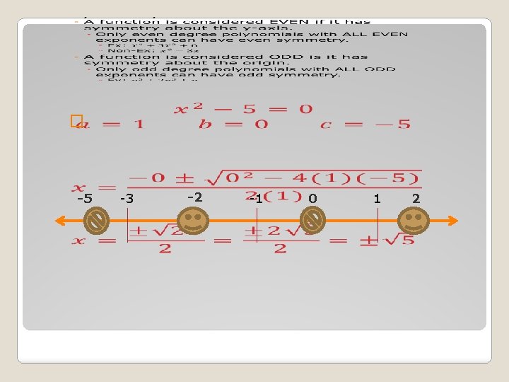
Steps 1. Set the polynomial equal to zero. 2. Solve the polynomial. Example �

3. Use the solutions to break up the number line. -3 -1 1

4. -5 Plug a “test point” from each section of the number in to the original inequality to test the validity of the value. -3 -2 -1 0 1 2