UNIT 4 PATHS PATH PRODUCTS AND REGULAR EXPRESSIONS

UNIT – 4 PATHS, PATH PRODUCTS AND REGULAR EXPRESSIONS MOTIVATION: o Flow graphs are being an abstract representation of programs. PATH PRODUCTS: o Normally flow graphs used to denote only control flow connectivity. o The simplest weight we can give to a link is a name.

o The link name will be denoted by lower case italic letters. o In tracing a path or path segment through a flow graph, you traverse a succession of link names. o For example, if you traverse links a, b, c and d along some path, the name for that path segment is abcd. This path name is also called a path product.

shows some examples: FIG: Examples of paths.

PATH EXPRESSION: o Consider a pair of nodes in a graph and the set of paths between those nodes. o Denote that set of paths by Upper case letter such as X, Y. From Figure c, the members of the path set can be listed as follows: ac, abbc, abbbbc. . . o Alternatively, the same set of paths can be denoted by : ac+abbc+abbbbc+. . .

o The + sign is understood to mean "or" between the two nodes of interest, paths ac, or abbc, and so on can be taken. o Any expression that consists of path names and "OR"s and which denotes a set of paths between two nodes is called a "Path Expression. " PATH PRODUCTS: The name of a path that consists of two successive path segments is conveniently expressed by the concatenation or Path Product of the segment names.

o For example, if X and Y are defined as X=abcde, Y=fghij, then the path corresponding to X followed by Y is denoted by XY=abcdefghij o Similarly, o YX=fghijabcde o a. X=aabcde o Xa=abcdea Xa. X=abcdeaabcde

o If X and Y represent sets of paths or path expressions, their product represents the set of paths that can be obtained by following every element of X by any element of Y in all possible ways. For example, o X = abc + def + ghi o Y = uvw + z Then, XY = abcuvw + defuvw + ghiuvw + abcz + defz + ghiz

o If a link or segment name is repeated, that fact is denoted by an exponent. The exponent's value denotes the number of repetitions: O a 1 = a; a 2 = aa; a 3 = aaa; an = aaaa. . . n times. Similarly, if X = abcde then X 1 = abcde X 2 = abcde = (abcde)2 X 3 = abcdeabcde = (abcde)2 abcde = abcde(abcde)2 = (abcde)3

o The path product is not commutative (that is XY!=YX). o The path product is Associative. RULE 1: A(BC)=(AB)C=ABC where A, B, C are path names, set of path names or path expressions. o The zeroth power of a link name, path product, or path expression is also needed for completeness. It is denoted by the numeral "1" and denotes the "path" whose length is zero - that is, the path that doesn't have any links. o a 0 = 1 o X 0 = 1

PATH SUMS: o The "+" sign was used to denote the fact that path names were part of the same set of paths. o The "PATH SUM" denotes paths in parallel between nodes. o Links a and b in Figure (a) are parallel paths and are denoted by a + b. Similarly, links c and d are parallel paths between the next two nodes and are denoted by c + d. o The set of all paths between nodes 1 and 2 can be thought of as a set of parallel paths and denoted by eacf+eadf+ebcf+ebdf. o If X and Y are sets of paths that lie between the same pair of nodes, then X+Y denotes the UNION of those set of paths.

Figure : Examples of path sums. The first set of parallel paths is denoted by X + Y + d and the second set by U + V + W + h + i + j. The set of all paths in this flowgraph is f(X + Y + d)g(U + V + W + h + i + j)k

o The path is a set union operation, it is clearly Commutative and Associative. o RULE 2: X+Y=Y+X o RULE 3: (X+Y)+Z=X+(Y+Z)=X+Y+Z DISTRIBUTIVE LAWS: o The product and sum operations are distributive, and the ordinary rules of multiplication apply; that is RULE 4: A(B+C)=AB+AC and (B+C)D=BD+CD o Applying these rules to the Figure 1(a) yields o e(a+b)(c+d)f=e(ac+ad+bc+bd)f = eacf+eadf+ebcf+ebdf

ABSORPTION RULE: o If X and Y denote the same set of paths, then the union of these sets is unchanged; consequently, RULE 5: X+X=X (Absorption Rule) LOOPS: o Loops can be understood as an infinite set of parallel paths.

Figure : Another example of path loops. o The path expression for the figure is denoted by the notation: ab*c=ac+abbc+abbbc+. . . . A bar is used under the exponent to denote the fact as follows: Xn = X 0+X 1+X 2+X 3+X 4+X 5+. . . . +Xn RULES 6 - 16: o The following rules can be derived from the previous rules: o RULE 6: Xn + Xm = Xn if n>m

RULE 7: Xn. Xm = Xn+m RULE 8: Xn. X* = X*Xn = X* RULE 9: Xn. X+ = X+Xn = X+ RULE 10: X*X+ = X+X* = X+ RULE 11: 1 + 1 = 1 RULE 12: 1 X = X 1 = X Following or preceding a set of paths by a path of zero length does not change the set. RULE 13: 1 n = 1* = 1+ = 1 No matter how often you traverse a path of zero length, It is a path of zero length. RULE 14: 1++1 = 1*=1 The null set of paths is denoted by the numeral 0. it obeys the following rules: RULE 15: X+0=0+X=X RULE 16: 0 X=X 0=0

REDUCTION PROCEDURE: REDUCTION PROCEDURE ALGORITHM: o This section presents a reduction procedure for converting a flowgraph whose links are labeled with names into a path expression that denotes the set of all entry/exit paths in that flowgraph. The procedure is a node-by-node removal algorithm. o The steps in Reduction Algorithm are as follows: 1. Combine all serial links by multiplying their path expressions. 2. Combine all parallel links by adding their path expressions. 3. Remove all self-loops (from any node to itself) by replacing them with a link of the form X*, where X is the path expression of the link in that loop.

STEPS 4 - 8 ARE IN THE ALGORIHTM'S LOOP: 4. Select any node for removal other than the initial or final node. Replace it with a set of equivalent links whose path expressions correspond to all the ways you can form a product of the set of inlinks with the set of outlinks of that node. 5. Combine any remaining serial links by multiplying their path expressions. 6. Combine all parallel links by adding their path expressions. 7. Remove all self-loops as in step 3. 8. Does the graph consist of a single link between the entry node and the exit node? If yes, then the path expression for that link is a path expression for the original flowgraph; otherwise, return to step 4.

LOOP REMOVAL OPERATIONS: o There are two ways of looking at the loopremoval operation: o In the first way, we remove the self-loop and then multiply all outgoing links by Z*.

o In the first way, we remove the self-loop and then multiply all outgoing links by Z*. o In the second way, we split the node into two equivalent nodes, call them A and A' and put in a link between them whose path expression is Z*. Then we remove node A' using steps 4 and 5 to yield outgoing links whose path expressions are Z*X and Z*Y.

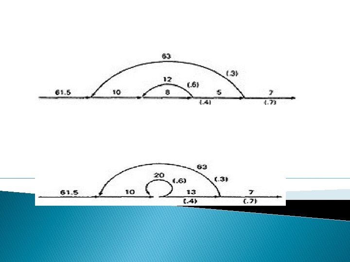
A REDUCTION PROCEDURE - EXAMPLE: o Let us see by applying this algorithm to the following graph where we remove several nodes in order; that is Figure : Example Flowgraph for demonstrating reduction procedure.

o Remove node 10 by applying step 4 and combine by step 5 to yield o Remove node 9 by applying step 4 and 5 to yield

o Remove node 7 by steps 4 and 5, as follows: o Remove node 8 by steps 4 and 5, to obtain:

o PARALLEL TERM (STEP 6): Removal of node 8 above led to a pair of parallel links between nodes 4 and 5. combine them to create a path expression for an equivalent link whose path expression is c+gkh; that is

o LOOP TERM (STEP 7): Removing node 4 leads to a loop term. The graph has now been replaced with the following equivalent simpler graph:

o Continue the process by applying the loop-removal step as follows o Removing node 5 produces: o Remove the loop at node 6 to yield:

o Remove node 3 to yield: o Removing the loop and then node 6 result in the following expression: o a(bgjf)*b(c+gkh)d((ilhd)*imf(bjgf)*b(c+gkh)d)*(i lhd)*e

� APPLICATIONS: o The purpose of the node removal algorithm is to present one very generalized concept- the path expression and way of getting it. o Every application follows this common pattern: 1. Convert the program or graph into a path expression. 2. Identify a property of interest and derive an appropriate set of "arithmetic" rules that characterizes the property. 3. Replace the link names by the link weights for the property of interest.

HOW MANY PATHS IN A FLOWGRAPH? o The question is not simple. Here are some ways you could ask it: 1. What is the maximum number of different paths possible? 2. What is the fewest number of paths possible? 3. How many different paths are there really? 4. What is the average number of paths?

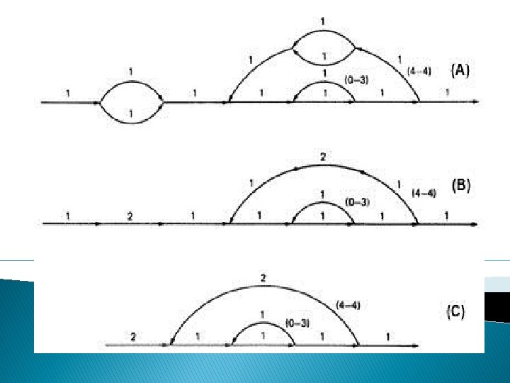
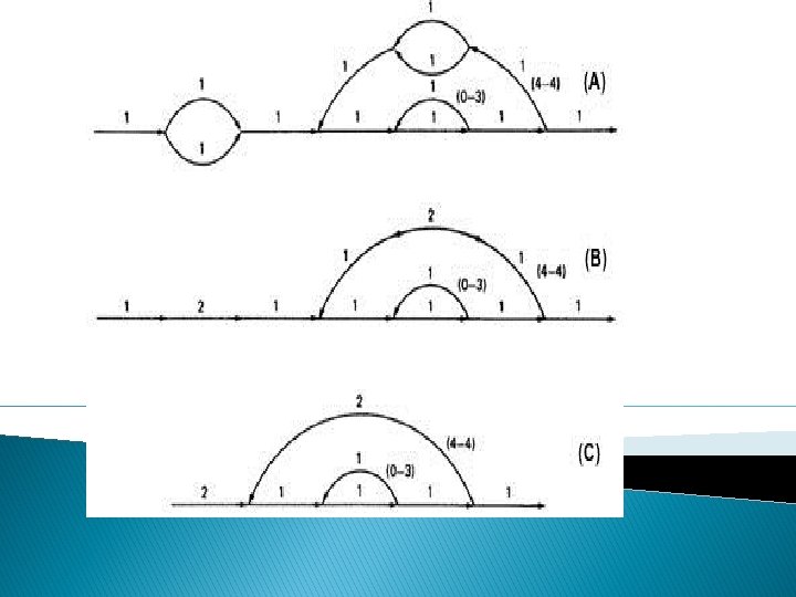
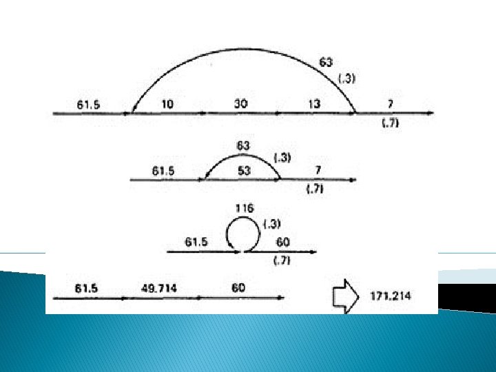
o EXAMPLE: The following is a reasonably well-structured program. Each link represents a single link and consequently is given a weight of "1" to start.

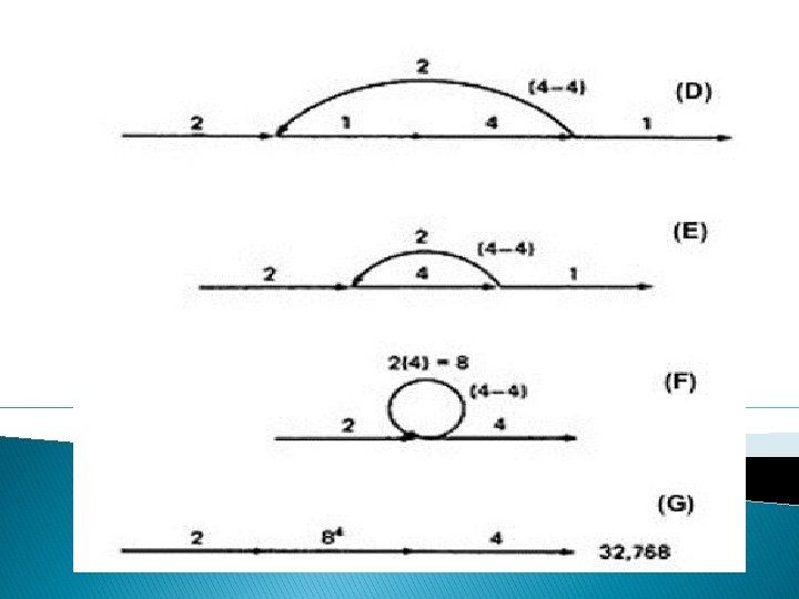
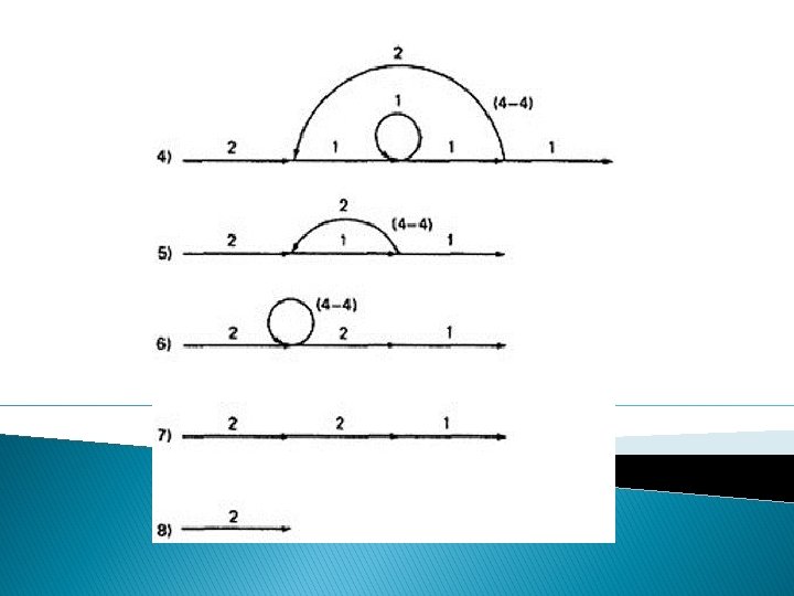
Path expression: a(b+c)d{e(fi)*fgj(m+l)k}*e(fi)*fgh � A: The flow graph should be annotated by replacing the link name with the maximum of paths through that link (1) and also note the number of times for looping. � B: Combine the first pair of parallel loops outside the loop and also the pair in the outer loop. � C: Multiply the things out and remove nodes to clear the clutter.

� For the Inner Loop: D: Calculate the total weight of inner loop, which can execute a min. of 0 times and max. of 3 times. So, it inner loop can be evaluated as follows: 13 = 10 + 11 + 12 + 13 = 1 + 1+1+1=4 � E: Multiply the link weights inside the loop: 1 X 4 =4 � F: Evaluate the loop by multiplying the link wieghts: 2 X 4 = 8. � G: Simpifying the loop further results in the total maximum number of paths in the flowgraph: 2 X 84 X 2 = 32, 768.

a(b+c)d{e(fi)*fgj(m+l)k}*e(fi)*fgh = 1(1 + 1)1(1(1 x 1)31 x 1(1 + 1)1)41(1 x 1)31 x 1 = 2(131 x (2))413 = 2(4 x 2)4 x 4 = 2 x 84 x 4 = 32, 768 STRUCTURED FLOWGRAPH: Structured code can be defined in several different ways that do not involve ad-hoc rules such as not using GOTOs. A structured flowgraph is one that can be reduced to a single link by successive application of the transformations of Figure

Figure : Structured Flowgraph Transformations

Flow graphs that DO NOT contain one or more of the graphs shown below (Figure 5. 8) as subgraphs are structured. 0. Jumping into loops 1. Jumping out of loops 2. Branching into decisions 3. Branching out of decisions

Figure : Un-structured sub-graphs.

LOWER PATH COUNT ARITHMETIC: A lower bound on the number of paths in a routine can be approximated for structured flow graphs. The values of the weights are the number of members in a set of paths.

EXAMPLE: � Applying the arithmetic to the earlier example gives us the identical steps until step 3 as below:

What is the probability of being at a certain point in a routine? We use the same algorithm as before: node-bynode removal of uninteresting nodes. Weights, Notations and Arithmetic: � Probabilities can come into the act only at decisions (including decisions associated with loops). � Annotate(=explain) each outlink with a weight equal to the probability of going in that direction.

� Evidently, the sum of the outlink probabilities must equal 1 � For a simple loop, if the loop will be taken a mean of N times, the looping probability is N/(N + 1) and the probability of not looping is 1/(N + 1) � A link that is not part of a decision node has a probability of 1.

� In this table, in case of a loop, PA is the probability of the link leaving the loop and PL is the probability of looping. 1. If you can do something either from column A with a probability of PA or from column B with a probability PB, then the probability that you do either is PA + PB. 2. For the series case, if you must do both things, and their probabilities are independent (as assumed), then the probability that you do both is the product of their probabilities.

� For example, a loop node has a looping probability of PL and a probability of not looping of PA, which is obviously equal to I - PL.

because PL + PA + PB + PC = 1, 1 - PL = PA + PB + PC, and

MEAN PROCESSING TIME OF A ROUTINE: The model has two weights associated with every link: the processing time for that link, denoted by T, and the probability of that link P.

EXAMPLE: 0. Start with the original flow graph annotated with probabilities and processing time.

PUSH/POP, GET/RETURN: Here are some other examples of complementary operations to which this model applies: GET/RETURN a resource block. OPEN/CLOSE a file. START/STOP a device or process. EXAMPLE 1 (PUSH / POP): � Here is the Push/Pop Arithmetic:

� The numeral 1 is used to indicate that nothing of interest (neither PUSH nor POP) occurs on a given link. � "H" denotes PUSH and "P" denotes POP. The operations are commutative, associative, and distributive.

� Consider the following flowgraph: P(P + 1)1{P(HH)n 1 HP 1(P + H)1}n 2 P(HH)n 1 HPH � Simplifying by using the arithmetic tables, =(P 2 + P){P(HH)n 1(P + H)}n 1(HH)n 1 =(P 2 + P){H 2 n 1(P 2 + 1)}n 2 H 2 n 1

LOGIC BASED TESTING: The functional requirements of many programs can be specified by decision tables, which provide a useful basis for program and test design. DECISION TABLES: � Following Figure is a limited - entry decision table. It consists of four areas called the condition stub (=end or remains), the condition entry, the action stub, and the action entry. � Each column of the table is a rule that specifies the conditions under which the actions named in the action stub will take place.

� The condition stub is a list of names of conditions.

1. A rule specifies whether a condition should or should not be met for the rule to be satisfied. "YES" means that the condition must be met, "NO" means that the condition must not be met, and "I" means that the condition plays no part in the rule, or it is immaterial (=irrelevant or unimportant) to that rule. a) Action 1 will take place if conditions 1 and 2 are met and if conditions 3 and 4 are not met (rule 1) or if conditions 1, 3, and 4 are met (rule 2).

� "Condition" is another word for predicate. b. Action 2 will be taken if the predicates are all false, (rule 3). c. Action 3 will take place if predicate 1 is false and predicate 4 is true (rule 4). � DECISION-TABLE PROCESSORS: o Decision tables can be automatically translated into code and, as such, are a higherorder language o If the rule is satisfied, the corresponding action takes place

Otherwise, rule 2 is tried. This process continues until either a satisfied rule results in an action or no rule is satisfied and the default action is taken DECISION-TABLES AND STRUCTURE: o Decision tables can also be used to examine a program's structure. o Figure shows a program segment that consists of a decision tree. o These decisions, in various combinations, can lead to actions 1, 2, or 3.

A Sample Program

o If the decision appears on a path, put in a YES or NO as appropriate. If the decision does not appear on the path, put in an I, Rule 1 does not contain decision C, therefore its entries are: YES, I, YES. o The corresponding decision table is shown in Table 6. 1

RULE 1 2 RULE 3 RULE 4 RULE 5 RULE 6 CONDITIO NA CONDITIO NB CONDITIO NC CONDITIO ND YES YES NO NO NO YES I I I YES NO NO YES I NO I YES NO ACTION 1 ACTION 2 ACTION 3 YES NO NO NO YES NO NO NO YES

o As an example, expanding the immaterial cases results as below:

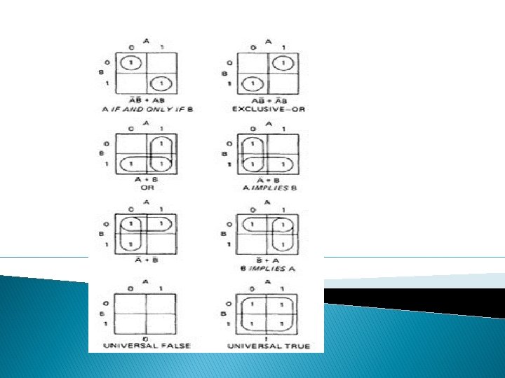
KV CHARTS: o Karnaugh-Veitch chart reduces boolean algebraic manipulations to graphical trivia. Figure : KV Charts for Functions of a Single Variable.

o The charts show all possible truth values that the variable A can have. A "1" means the variable’s value is "1" or TRUE. A "0" means that the variable's value is 0 or FALSE. o The entry in the box (0 or 1) specifies whether the function that the chart represents is true or false for that value of the variable.

� TWO VARIABLES

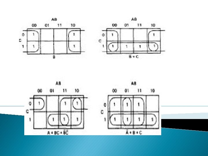
� THREE VARIABLES: