Unit 4 OBST 1 Greedy Method 2 Greedy

Unit - 4 OBST 1
Greedy Method 2

Greedy Method Greedy Principal: are typically used to solve optimization problem. Most of these problems have n inputs and require us to obtain a subset that satisfies some constraints. Any subset that satisfies these constraints is called a feasible solution. We are required to find a feasible solution that either minimizes or maximizes a given objective function. In the most common situation we have:
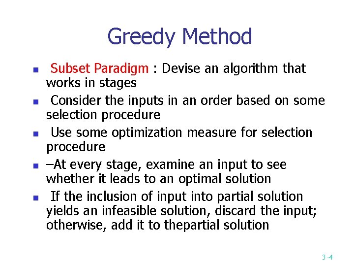
Greedy Method Subset Paradigm : Devise an algorithm that works in stages Consider the inputs in an order based on some selection procedure Use some optimization measure for selection procedure –At every stage, examine an input to see whether it leads to an optimal solution If the inclusion of input into partial solution yields an infeasible solution, discard the input; otherwise, add it to thepartial solution 3 -4
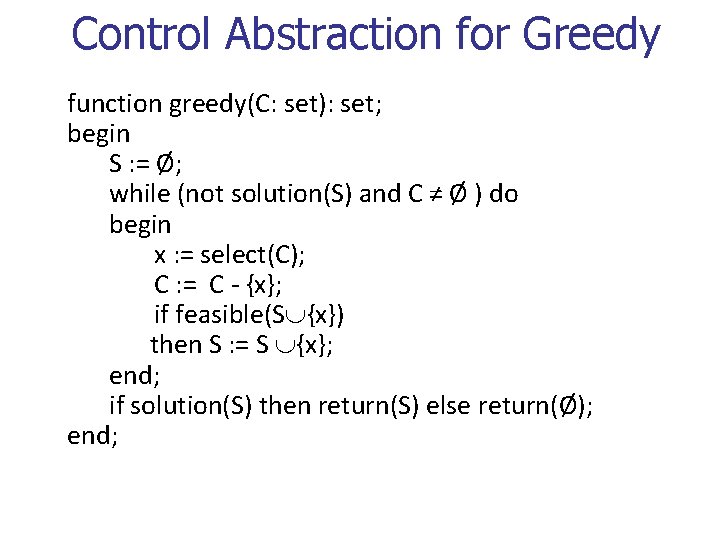
Control Abstraction for Greedy function greedy(C: set): set; begin S : = Ø; while (not solution(S) and C ≠ Ø ) do begin x : = select(C); C : = C - {x}; if feasible(S {x}) then S : = S {x}; end; if solution(S) then return(S) else return(Ø); end;
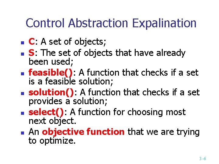
Control Abstraction Expalination C: A set of objects; S: The set of objects that have already been used; feasible(): A function that checks if a set is a feasible solution; solution(): A function that checks if a set provides a solution; select(): A function for choosing most next object. An objective function that we are trying to optimize. 3 -6
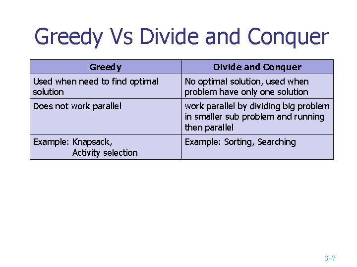
Greedy Vs Divide and Conquer Greedy Divide and Conquer Used when need to find optimal solution No optimal solution, used when problem have only one solution Does not work parallel by dividing big problem in smaller sub problem and running then parallel Example: Knapsack, Activity selection Example: Sorting, Searching 3 -7

Knapsack problem using Greedy Method 8
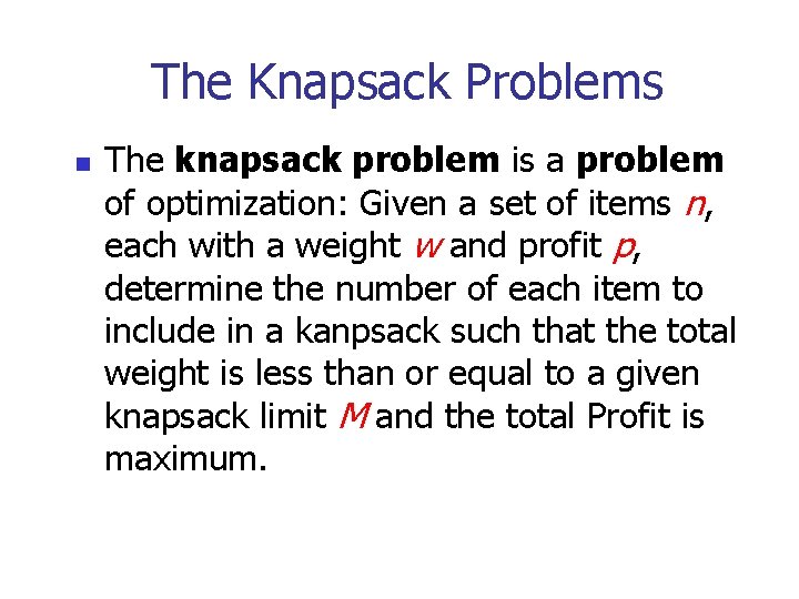
The Knapsack Problems The knapsack problem is a problem of optimization: Given a set of items n, each with a weight w and profit p, determine the number of each item to include in a kanpsack such that the total weight is less than or equal to a given knapsack limit M and the total Profit is maximum.
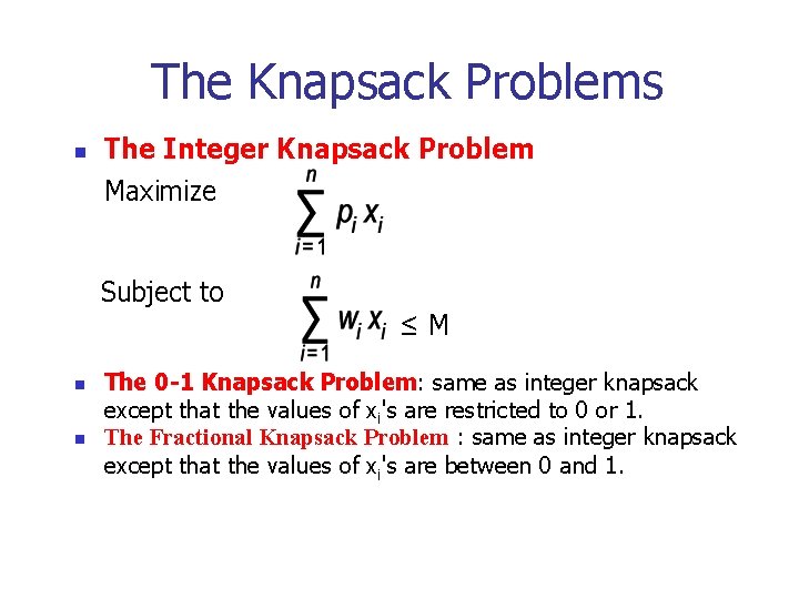
The Knapsack Problems The Integer Knapsack Problem Maximize Subject to ≤M The 0 -1 Knapsack Problem: same as integer knapsack except that the values of xi's are restricted to 0 or 1. The Fractional Knapsack Problem : same as integer knapsack except that the values of xi's are between 0 and 1.
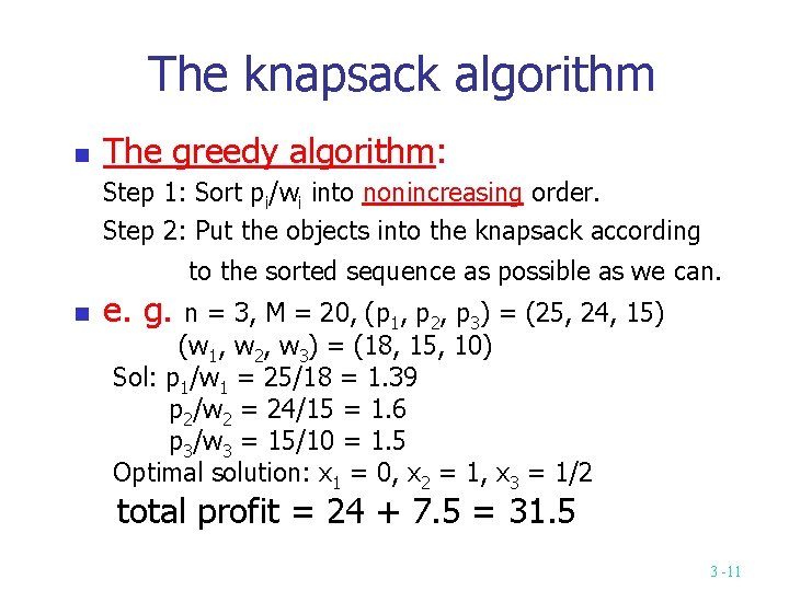
The knapsack algorithm The greedy algorithm: Step 1: Sort pi/wi into nonincreasing order. Step 2: Put the objects into the knapsack according to the sorted sequence as possible as we can. e. g. n = 3, M = 20, (p 1, p 2, p 3) = (25, 24, 15) (w 1, w 2, w 3) = (18, 15, 10) Sol: p 1/w 1 = 25/18 = 1. 39 p 2/w 2 = 24/15 = 1. 6 p 3/w 3 = 15/10 = 1. 5 Optimal solution: x 1 = 0, x 2 = 1, x 3 = 1/2 total profit = 24 + 7. 5 = 31. 5 3 -11
Job sequencing using Greedy Method 12
JOB SEQUENCING WITH DEADLINES The problem is stated as below. There are n jobs to be processed on a machine. Each job i has a deadline di≥ 0 and profit pi≥ 0. Pi is earned iff the job is completed by its deadline. The job is completed if it is processed on a machine for unit time. Only one machine is available for processing jobs. Only one job is processed at a time on the machine. 13
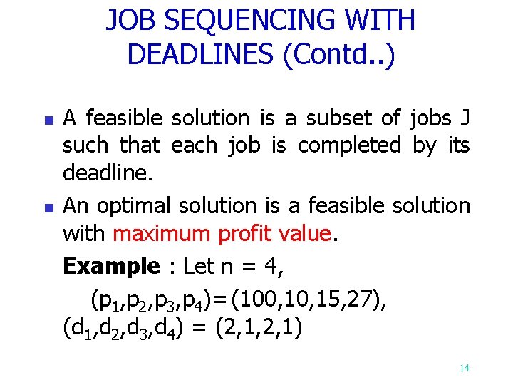
JOB SEQUENCING WITH DEADLINES (Contd. . ) A feasible solution is a subset of jobs J such that each job is completed by its deadline. An optimal solution is a feasible solution with maximum profit value. Example : Let n = 4, (p 1, p 2, p 3, p 4)= (100, 15, 27), (d 1, d 2, d 3, d 4) = (2, 1, 2, 1) 14
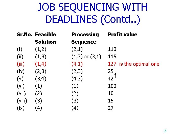
JOB SEQUENCING WITH DEADLINES (Contd. . ) Sr. No. Feasible Solution (i) (1, 2) (ii) (1, 3) (iii) (1, 4) (iv) (2, 3) (v) (3, 4) (vi) (1) (vii) (2) (viii) (3) (ix) (4) Processing Sequence (2, 1) (1, 3) or (3, 1) (4, 1) (2, 3) (4, 3) (1) (2) (3) (4) Profit value 110 115 127 is the optimal one 25 42 100 10 15 27 15
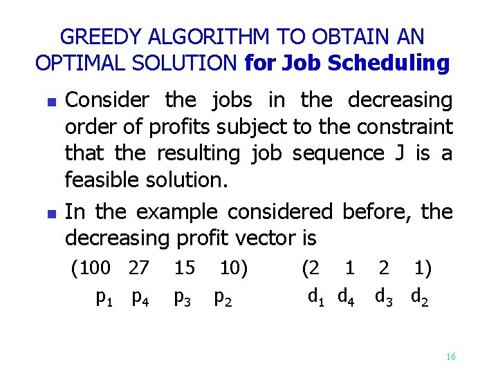
GREEDY ALGORITHM TO OBTAIN AN OPTIMAL SOLUTION for Job Scheduling Consider the jobs in the decreasing order of profits subject to the constraint that the resulting job sequence J is a feasible solution. In the example considered before, the decreasing profit vector is (100 27 p 1 p 4 15 10) p 3 p 2 (2 1 d 4 2 1) d 3 d 2 16
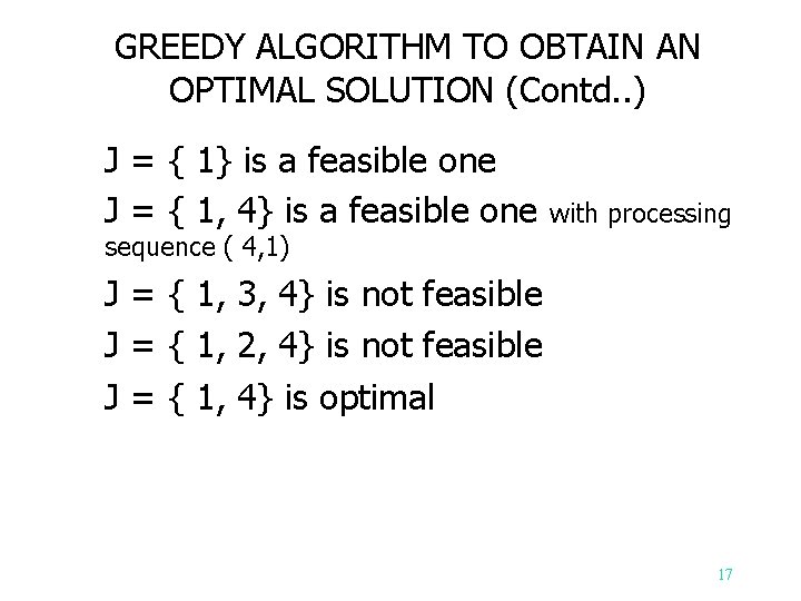
GREEDY ALGORITHM TO OBTAIN AN OPTIMAL SOLUTION (Contd. . ) J = { 1} is a feasible one J = { 1, 4} is a feasible one with processing sequence ( 4, 1) J = { 1, 3, 4} is not feasible J = { 1, 2, 4} is not feasible J = { 1, 4} is optimal 17
Activity Selection Using Greedy Method 18
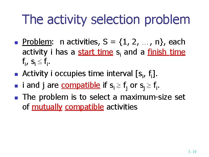
The activity selection problem Problem: n activities, S = {1, 2, …, n}, each activity i has a start time si and a finish time fi, s i fi. Activity i occupies time interval [si, fi]. i and j are compatible if si fj or sj fi. The problem is to select a maximum-size set of mutually compatible activities 3 -19
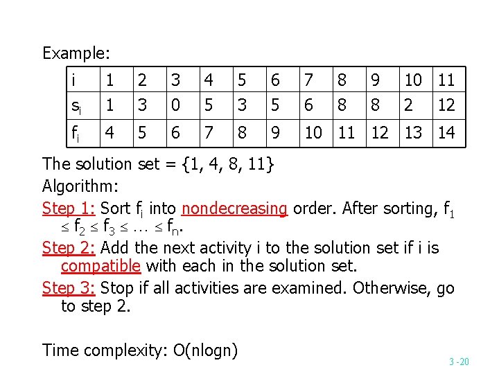
Example: i 1 2 3 4 5 6 7 8 9 10 11 si 1 3 0 5 3 5 6 8 8 2 fi 4 5 6 7 8 9 10 11 12 13 14 12 The solution set = {1, 4, 8, 11} Algorithm: Step 1: Sort fi into nondecreasing order. After sorting, f 1 f 2 f 3 … f n. Step 2: Add the next activity i to the solution set if i is compatible with each in the solution set. Step 3: Stop if all activities are examined. Otherwise, go to step 2. Time complexity: O(nlogn) 3 -20
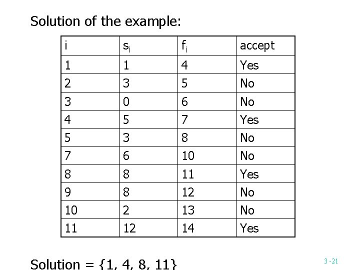
Solution of the example: i si fi accept 1 1 4 Yes 2 3 5 No 3 0 6 No 4 5 7 Yes 5 3 8 No 7 6 10 No 8 8 11 Yes 9 8 12 No 10 2 13 No 11 12 14 Yes Solution = {1, 4, 8, 11} 3 -21
Dynamic programming 22
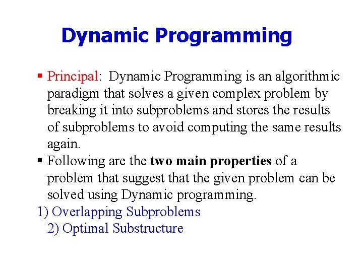
Dynamic Programming Principal: Dynamic Programming is an algorithmic paradigm that solves a given complex problem by breaking it into subproblems and stores the results of subproblems to avoid computing the same results again. Following are the two main properties of a problem that suggest that the given problem can be solved using Dynamic programming. 1) Overlapping Subproblems 2) Optimal Substructure
Dynamic Programming 1) Overlapping Subproblems: Dynamic Programming is mainly used when solutions of same subproblems are needed again and again. In dynamic programming, computed solutions to subproblems are stored in a table so that these don’t have to recomputed. 2) Optimal Substructure: A given problems has Optimal Substructure Property if optimal solution of the given problem can be obtained by using optimal solutions of its subproblems. 3 -24
The principle of optimality Dynamic programming is a technique for finding an optimal solution The principle of optimality applies if the optimal solution to a problem always contains optimal solutions to all subproblems 25
Differences between Greedy, D&C and Dynamic Greedy. Build up a solution incrementally, myopically optimizing some local criterion. Divide-and-conquer. Break up a problem into two sub-problems, solve each subproblem independently, and combine solution to sub-problems to form solution to original problem. Dynamic programming. Break up a problem into a series of overlapping sub-problems, and build up solutions to larger and larger sub -problems. 26
Divide and conquer Vs Dynamic Programming Divide-and-Conquer: a top-down approach. Many smaller instances are computed more than once. Dynamic programming: a bottom-up approach. Solutions for smaller instances are stored in a table for later use.
0/1 knapsack using Dynamic Programming 28
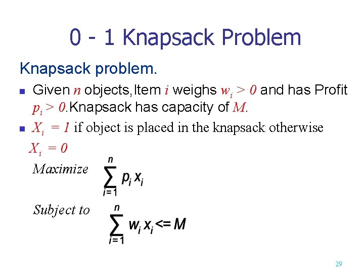
0 - 1 Knapsack Problem Knapsack problem. Given n objects, Item i weighs wi > 0 and has Profit pi > 0. Knapsack has capacity of M. Xi = 1 if object is placed in the knapsack otherwise Xi = 0 Maximize Subject to 29
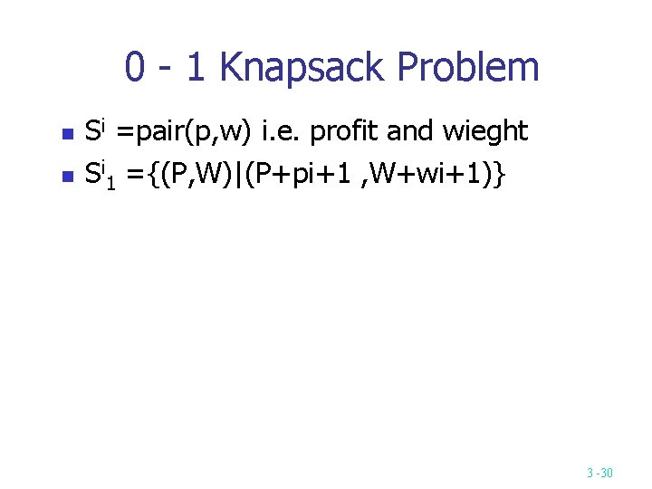
0 - 1 Knapsack Problem Si =pair(p, w) i. e. profit and wieght Si 1 ={(P, W)|(P+pi+1 , W+wi+1)} 3 -30
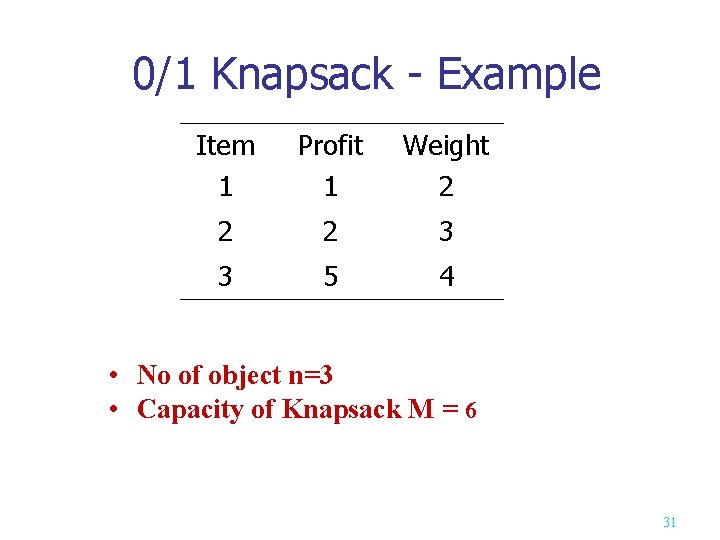
0/1 Knapsack - Example Item 1 Profit 1 Weight 2 2 2 3 3 5 4 • No of object n=3 • Capacity of Knapsack M = 6 31
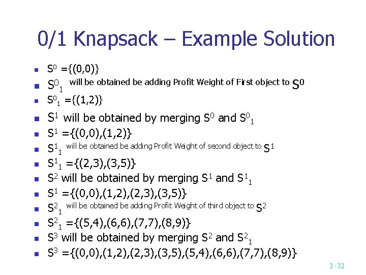
0/1 Knapsack – Example Solution S 0 ={(0, 0)} S 0 1 will be obtained be adding Profit Weight of First object to S 01 ={(1, 2)} S 1 will be obtained by merging S 0 and S 01 S 1 ={(0, 0), (1, 2)} S 11 will be obtained be adding Profit Weight of second object to S 11 ={(2, 3), (3, 5)} S 2 will be obtained by merging S 1 and S 11 S 1 ={(0, 0), (1, 2), (2, 3), (3, 5)} S 21 will be obtained be adding Profit Weight of third object to S 21 ={(5, 4), (6, 6), (7, 7), (8, 9)} S 3 will be obtained by merging S 2 and S 21 S 3 ={(0, 0), (1, 2), (2, 3), (3, 5), (5, 4), (6, 6), (7, 7), (8, 9)} 3 -32
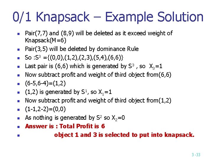
0/1 Knapsack – Example Solution Pair(7, 7) and (8, 9) will be deleted as it exceed weight of Knapsack(M=6) Pair(3, 5) will be deleted by dominance Rule So : S 3 ={(0, 0), (1, 2), (2, 3), (5, 4), (6, 6)} Last pair is (6, 6) which is generated by S 3 , so X 3=1 Now subtract profit and weight of third object from(6, 6) (6 -5, 6 -4)=(1, 2) is generated by S 1, so X 1=1 Now subtract profit and weight of third object from(1, 2) (1 -1, 2 -2)=(0, 0) As nothing is generated by S 2 so X 2=0 Answer is : Total Profit is 6 object 1 and 3 is selected to put into knapsack. 3 -33

Binomial Coefficient using Dynamic Programming 34
The Binomial Coefficient D. P. 35
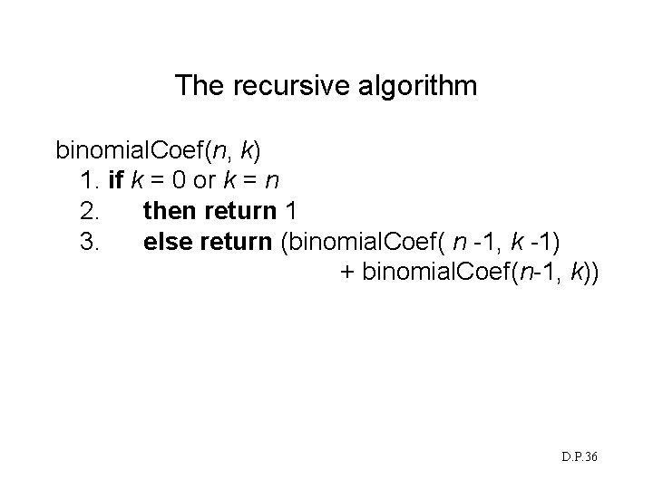
The recursive algorithm binomial. Coef(n, k) 1. if k = 0 or k = n 2. then return 1 3. else return (binomial. Coef( n -1, k -1) + binomial. Coef(n-1, k)) D. P. 36
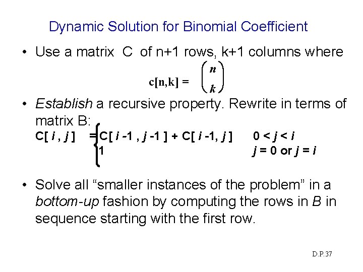
Dynamic Solution for Binomial Coefficient • Use a matrix C of n+1 rows, k+1 columns where c[n, k] = n k • Establish a recursive property. Rewrite in terms of matrix B: C[ i , j ] = C[ i -1 , j -1 ] + C[ i -1, j ] 1 0<j<i j = 0 or j = i • Solve all “smaller instances of the problem” in a bottom-up fashion by computing the rows in B in sequence starting with the first row. D. P. 37
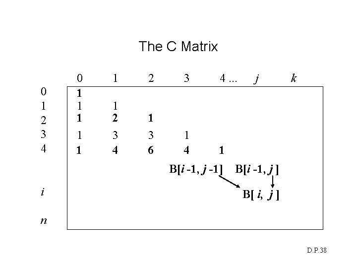
The C Matrix 0 1 2 3 4 0 1 1 1 2 3 4. . . 1 2 3 4 1 3 6 1 4 1 B[i -1, j -1] i j k B[i -1, j ] B[ i, j ] n D. P. 38
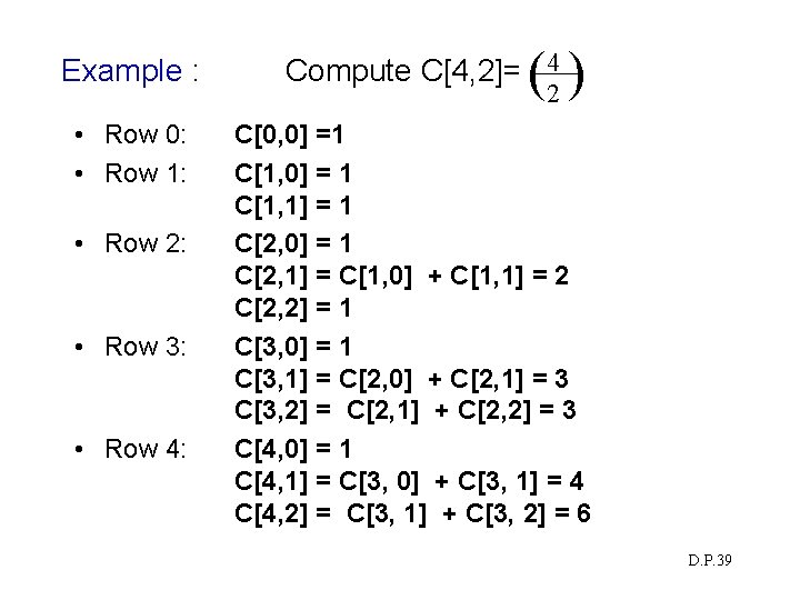
Example : • Row 0: • Row 1: • Row 2: • Row 3: • Row 4: (2 ) Compute C[4, 2]= 4 C[0, 0] =1 C[1, 0] = 1 C[1, 1] = 1 C[2, 0] = 1 C[2, 1] = C[1, 0] + C[1, 1] = 2 C[2, 2] = 1 C[3, 0] = 1 C[3, 1] = C[2, 0] + C[2, 1] = 3 C[3, 2] = C[2, 1] + C[2, 2] = 3 C[4, 0] = 1 C[4, 1] = C[3, 0] + C[3, 1] = 4 C[4, 2] = C[3, 1] + C[3, 2] = 6 D. P. 39
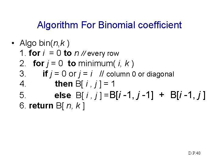
Algorithm For Binomial coefficient • Algo bin(n, k ) 1. for i = 0 to n // every row 2. for j = 0 to minimum( i, k ) 3. if j = 0 or j = i // column 0 or diagonal 4. then B[ i , j ] = 1 5. else B[ i , j ] =B[i -1, j -1] + B[i -1, j ] 6. return B[ n, k ] D. P. 40
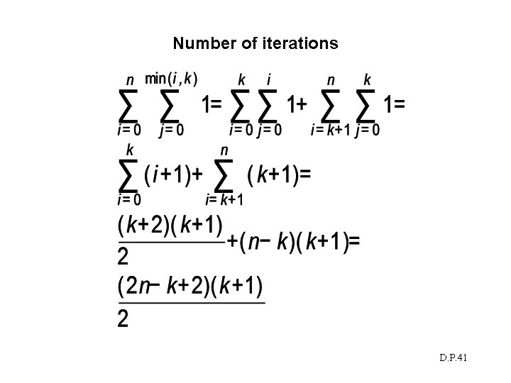
Number of iterations D. P. 41
Optimal Binary Search Tree (OBST) using Dynamic Programming 42
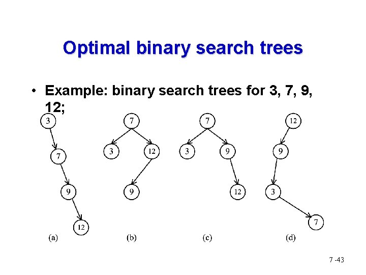
Optimal binary search trees • Example: binary search trees for 3, 7, 9, 12; 7 -43
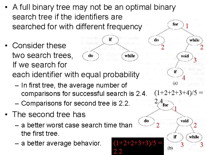
• A full binary tree may not be an optimal binary search tree if the identifiers are searched for with different frequency • Consider these two search trees, If we search for each identifier with equal probability – In first tree, the average number of comparisons for successful search is 2. 4. – Comparisons for second tree is 2. 2. • The second tree has 1 2 2 3 4 (1+2+2+3+4)/5 = 2. 4 1 – a better worst case search time than 2 the first tree. (1+2+2+3+3)/5 = – a better average behavior. 2. 2 2 3 3
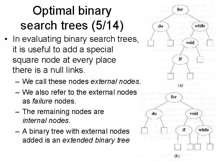
Optimal binary search trees (5/14) • In evaluating binary search trees, it is useful to add a special square node at every place there is a null links. – We call these nodes external nodes. – We also refer to the external nodes as failure nodes. – The remaining nodes are internal nodes. – A binary tree with external nodes added is an extended binary tree
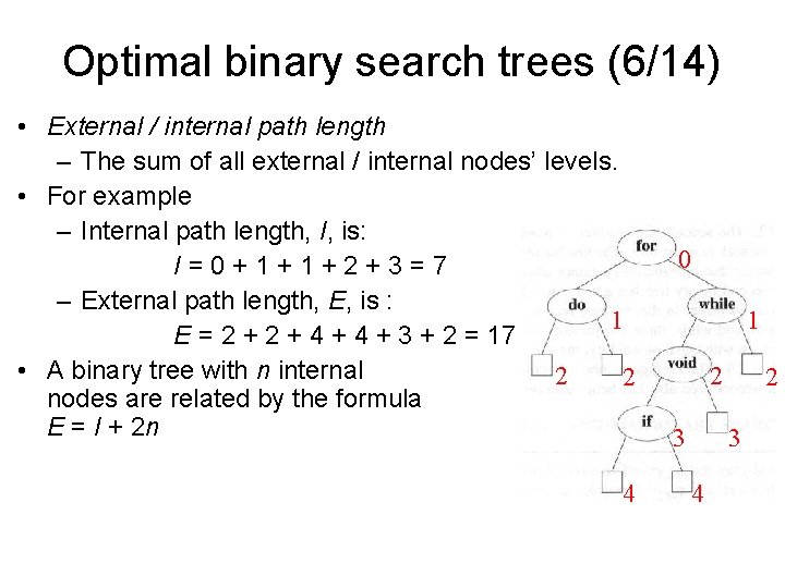
Optimal binary search trees (6/14) • External / internal path length – The sum of all external / internal nodes’ levels. • For example – Internal path length, I, is: I=0+1+1+2+3=7 – External path length, E, is : 1 E = 2 + 4 + 3 + 2 = 17 • A binary tree with n internal 2 2 nodes are related by the formula E = I + 2 n 4 0 1 2 3 4
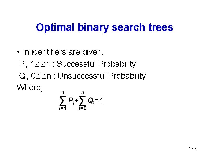
Optimal binary search trees • n identifiers are given. Pi, 1 i n : Successful Probability Qi, 0 i n : Unsuccessful Probability Where, 7 -47
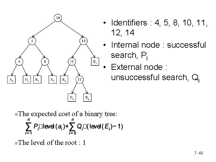
• Identifiers : 4, 5, 8, 10, 11, 12, 14 • Internal node : successful search, Pi • External node : unsuccessful search, Qi The expected cost of a binary tree: The level of the root : 1 7 -48
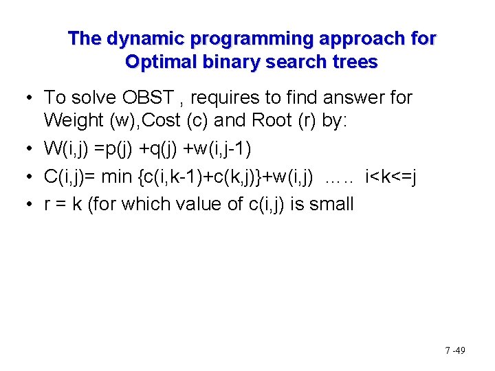
The dynamic programming approach for Optimal binary search trees • To solve OBST , requires to find answer for Weight (w), Cost (c) and Root (r) by: • W(i, j) =p(j) +q(j) +w(i, j-1) • C(i, j)= min {c(i, k-1)+c(k, j)}+w(i, j) …. . i<k<=j • r = k (for which value of c(i, j) is small 7 -49
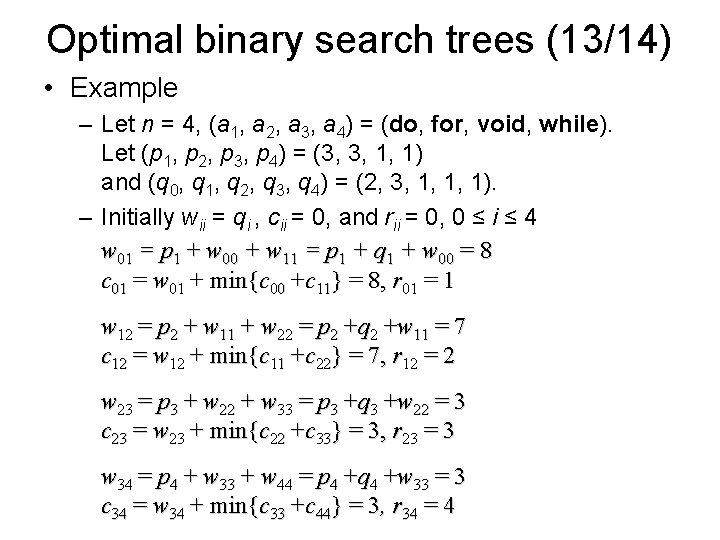
Optimal binary search trees (13/14) • Example – Let n = 4, (a 1, a 2, a 3, a 4) = (do, for, void, while). Let (p 1, p 2, p 3, p 4) = (3, 3, 1, 1) and (q 0, q 1, q 2, q 3, q 4) = (2, 3, 1, 1, 1). – Initially wii = qi , cii = 0, and rii = 0, 0 ≤ i ≤ 4 w 01 = p 1 + w 00 + w 11 = p 1 + q 1 + w 00 = 8 c 01 = w 01 + min{c 00 +c 11} = 8, r 01 = 1 w 12 = p 2 + w 11 + w 22 = p 2 +q 2 +w 11 = 7 c 12 = w 12 + min{c 11 +c 22} = 7, r 12 = 2 w 23 = p 3 + w 22 + w 33 = p 3 +q 3 +w 22 = 3 c 23 = w 23 + min{c 22 +c 33} = 3, r 23 = 3 w 34 = p 4 + w 33 + w 44 = p 4 +q 4 +w 33 = 3 c 34 = w 34 + min{c 33 +c 44} = 3, r 34 = 4
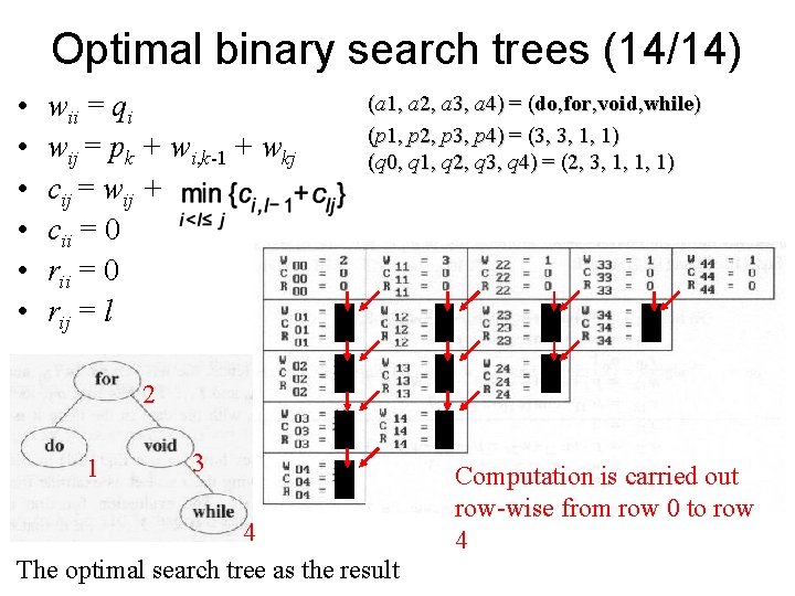
Optimal binary search trees (14/14) • • • wii = qi wij = pk + wi, k-1 + wkj cij = wij + cii = 0 rij = l (a 1, a 2, a 3, a 4) = (do, for, void, while) (p 1, p 2, p 3, p 4) = (3, 3, 1, 1) (q 0, q 1, q 2, q 3, q 4) = (2, 3, 1, 1, 1) 2 1 3 4 The optimal search tree as the result Computation is carried out row-wise from row 0 to row 4
Chain Matrix Multiplication using Dynamic Programming 52
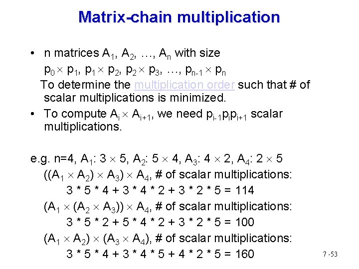
Matrix-chain multiplication • n matrices A 1, A 2, …, An with size p 0 p 1, p 1 p 2, p 2 p 3, …, pn-1 pn To determine the multiplication order such that # of scalar multiplications is minimized. • To compute Ai Ai+1, we need pi-1 pipi+1 scalar multiplications. e. g. n=4, A 1: 3 5, A 2: 5 4, A 3: 4 2, A 4: 2 5 ((A 1 A 2) A 3) A 4, # of scalar multiplications: 3 * 5 * 4 + 3 * 4 * 2 + 3 * 2 * 5 = 114 (A 1 (A 2 A 3)) A 4, # of scalar multiplications: 3 * 5 * 2 + 5 * 4 * 2 + 3 * 2 * 5 = 100 (A 1 A 2) (A 3 A 4), # of scalar multiplications: 3 * 5 * 4 + 3 * 4 * 5 + 4 * 2 * 5 = 160 7 -53
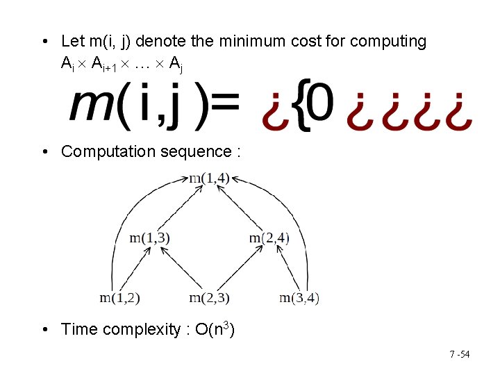
• Let m(i, j) denote the minimum cost for computing Ai Ai+1 … Aj • Computation sequence : • Time complexity : O(n 3) 7 -54
- Slides: 54