UNIT 4 NETWORK ARCHITECTURE Comparison between Architecture and

UNIT 4 NETWORK ARCHITECTURE

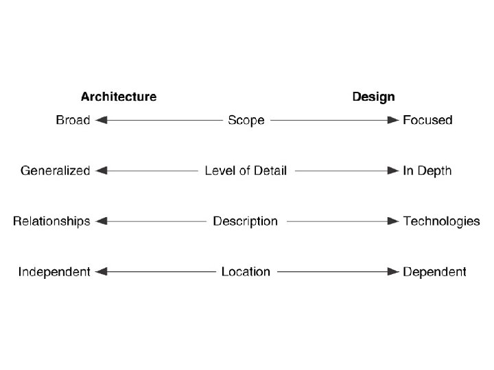
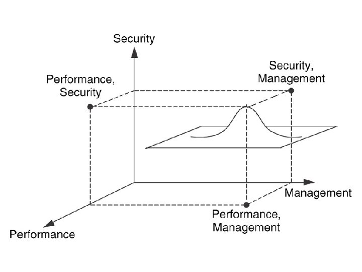
Comparison between Architecture and design Architecture Design 1. Scope is broad 1. Gives a detailed description 2. Gives a high level view of the network including locations of major components 2. Gives details of each portion of the network 3. Architecture relationships about 3. Design specifies technologies, protocols and network evices 4. Some parts of the architecture are location dependent like , external interfaces , relationships between components are location independent 4. Location information is important for design process describes Similarity is that both architecture and design attempt to solve multi dimensional problems , where the variables could be performance, security and network management

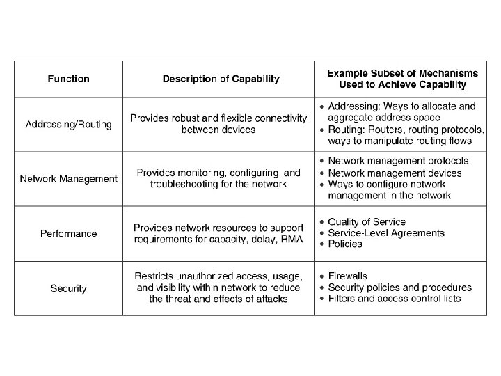
Component Architecture 1. Component Architecture is the description of how and where each function of a network is applied within that network. It consists of a set of mechanisms , by which that function is applied to the network, and a set of internal relationships between these mechanisms 2. Functions of a network represent major capabilities like addressing and routing, network management , performance and security 3. Mechanisms are h/w or s/w that help a n/w achieve each capabilities 4. Internal relationships consist of interactions , protocols and messages and are used to optimize each function within the network. 5. Tradeoff’s are decision points in the development of the network 6. Dependencies occur when mech. Relies on another for its operation. 7. Constraints are restrictions that one mech. , places on another.

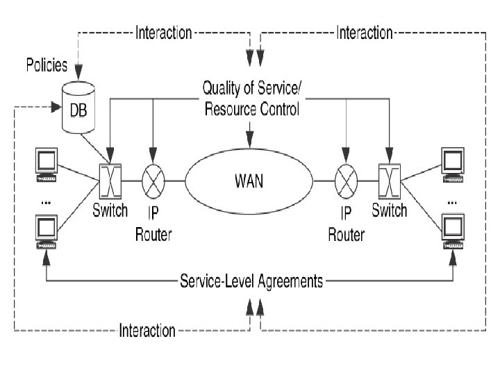
• In developing a component architecture consists of determining the mechanisms that make up each component, how the mechanisms work and how that component works as a whole For Example : to develop the component performance component Performance Qo. S Service Level Agreement mechanisms Policies

1. Qo. S is applied to each network device to control its resources in support of its SLA and policies 2. SLA ties subscribers to service levels 3. Policies provide high level of frame work for service levels , SLA’s and Qo. S A Service Level Agreement (SLA) is a formal definition of the relationship that exists between a service provider and its customer. A SLA can be defined and used in the context of any industry, and is used to specify what the customer could expect from the provider, the obligations of the customer as well as the provider, performance, availability and security objectives of the service, as well as the procedures to be followed to ensure compliance with the SLA

Addressing/ Routing Component Architecture 1. Addressing is applying addresses / identifiers to devices at various protocol layers 2. Routing is learning about the connectivity within and between the networks and applying this connectivity to forward IP packets towards their destinations 3. This component architecture determines A) How user , management traffic flows are prapagated. B) Determines the degree and diversity in the network C) How areas of the network can be divided MECHANISMS ADDRESSING MECHANISMS ROUTING MECHANISMS

ADDRESSING MECHANISMS PRIVATE ADDRESSING VARIABLE LENGTH SUBNETTNG SUPERNETTING DYNAMIC ADDRESSING VIRTUAL LANS IPv 6 NAT SUBNETTING

Routing mechanisms SWITCHING AND ROUTING MULTICASTS DEFAULT ROUTTE PROPAGATION MOBILE IP CIDR ROUTE FILTERING ROUTING POLICIES PEERING IGP AND EGP SELECTION AND LOCATION

Network Management Component and Architecture 1. It provides functions to control, plan , allocate , deploy , co-ordinate and monitor network resources 2. NMA is important as it determines how and where management mechanisms are applied in the network 3. Other architectural components require interactions with NMA 4. It describes how other network functions are monitored and managed Network Management Mechanisms Monitoring Instrumentation Configuration Scaling network management traffic FCAPS Integration into OSS MIB selection Checks and balances Managing network management data Centralised and distributed management Inband outband Management

PERFORMANCE COMPONENT ARCHITECTURE 1. Performance consists of the set of mechanisms used to configure , operate manage provision and account for resources in the network that allocate performance to users, applications and devices 2. Performances applies at multiple layers 3. This component describes how resources are allocated to user and management traffic flows 4. Prioritizing, scheduling and conditioning traffic flows are part of the duties of this component. Co-relation between users, applications and devices to traffic flow, traffic engineering, access control, quality of service policies and SLA are the other mechanisms used in this component

Security component Architecture 1. Security is a requirement to guarantee the confidentiality, integrity, and availability of users, applications , devices and network information and physical resources 2. This component also provides privacy 3. This component describes how system resources are to be protected from theft, damage, Do. S, or unauthorized access 4. These mechanisms can be targeted towards specific areas of the network , such as external interfaces, aggregation points or at devices …etc 4. This component determines to what level of security and privacy are needed, where the critical areas are and how it will impact and interact with other architectural components Mechanisms Security threat analysis protocol and application security Security policies and procedures Physical security and awareness Remote access security Encryption Network perimeter security

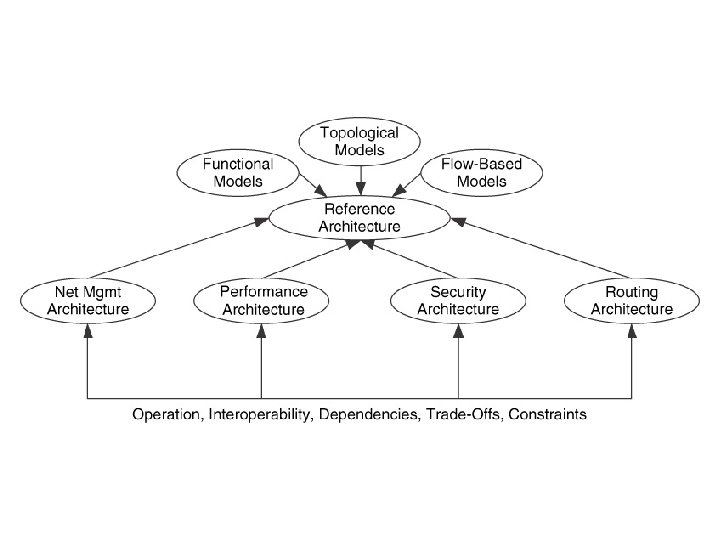
Reference Architecture 1. It is a description of the complete network architecture and contains all of the component architectures being considered for that network 2. Compilation of the internal and external architectures 3. Once the component architectures are determined their relationships with one another are determined 4. It incorporates the effects that functions have on one another 5. Based on the requirements , traffic flows and goals , the reference architecture is either b lanced or weighted. 6. In a balanced architecture all functions , constraints and dependencies are minimized , trade offs between functions are balances so that no individual function is prioritized over the other 7. When one or more functions are prioritized over the others , the external relationship between these functions and the other functions would be weighted in favor of this function

1. To develop component architectures requires input from sets of users, applications and device requirements, estimated traffic flow and architectural goals 2. For ex: user application and device requirements are used as criteria to evaluate mechanisms for the performance and security component architectures 3. Component architectures , requirements , flows and goals are all interwoven through the reference architecture
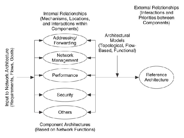

External Relationships 1. External Relationships define the relationships between different functions within a network as well as the requirements from the users , applications and devices. 2. The addressing and routing component architecture supports traffic flow from each and every other function OPTIMIZING THE REFERENCE ARCHITECTURE 1. Interaction between performance and security 2. Interaction between network management and security 3. Interaction between network management and performance 4. Interaction between addressing / routing and performance

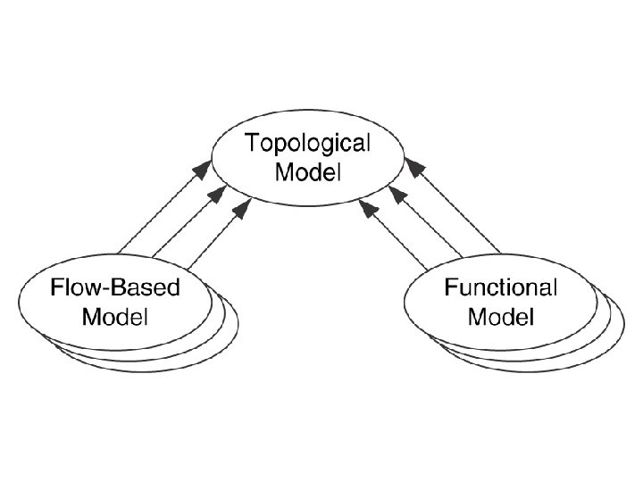
Architectural Models In developing the architectural models there are three types of models 1. Topological models 2. Flow based models 3. Functional models Topological models 1. These are based on geographical or topological arrangement 2. there are two models a) LAN/MAN/WAN model b) Access/Distribution/Core model LAN/MAN/WAN model 1. It is based on the geographical or topological distances between the networks 2. It focuses on the features and requirements of these boundaries 3. Compartmentalising functions , services , performances and features of the network along those boundaries 4. They indicate the hierarchy needed in the network Access/Distribution/Core model 1. It compartmentalises similar to lan model 2. It focuses on functions rather than on locations

LAN/MAN/WAN model

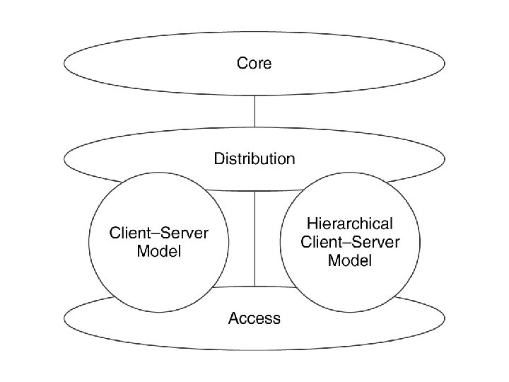
Access/Distribution/Core model

3. It reflects the behaviour of the network at its access, distribution and core areas 4. Access areas are closest to the users and it is these areas that most of the traffic is sourced and sinked 5. Distribution areas are most likely to be to or from multiple – user devices such as servers or specialised devices 6. The core of the network is used for bulk transport of the traffic, and flows are usually not sources or sinked at the core

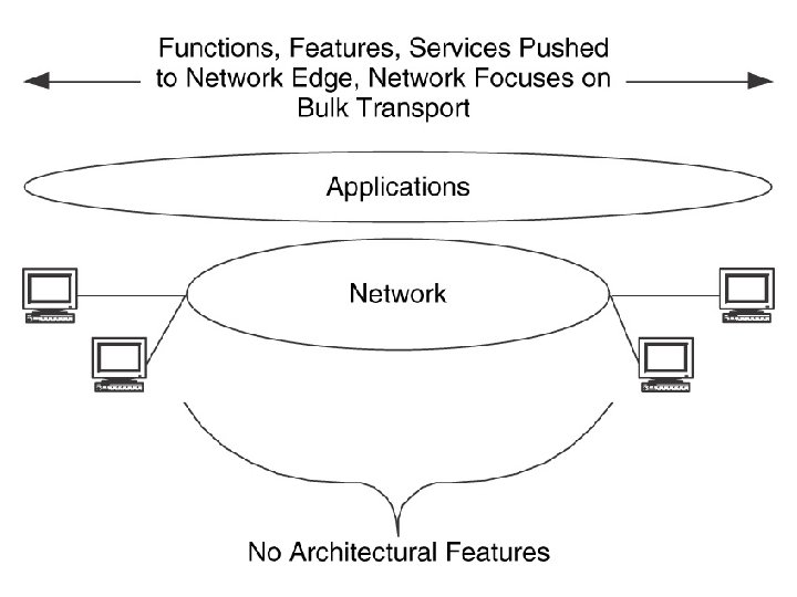
Flow Based Models 1. The flow based architectural models are based on the flow based model used in analysis 2. The peer to peer architectural model is based on the peer to peer flow model , where the users and their applications are fairly consistent in their behaviours 3. This pushes the functions, features and services towards the edge of the network 4. This resembles the core portion of the access/ Distribution/Core model 5. The client server architectural model also follows its flow model, but in this case there are obvious locations for architectural features—i. e where flows combine 6. Functions/ features and services are focussed at server locations, interfaces to client LAN and client server flows 7. Hierarchical client server models these Functions/ features and services are also focussed at server-server flows 8. In distributed computing architectural model the data sources and sinks are obvious locations for architectural features

CLIENT SERVER MODEL

HIERARCHICAL CLIENT SERVER MODEL

Distributed Computing Architecture Model

Functional Models 1. Functional Architectural models focus on supporting particular functions in the network 2. In the service provider architectural model , functions focus on privacy, security , service delivery , and billing 3. In the intranet and extranet architectural models security and privacy including the separation of users, devices and applications based on secure access are focused 4. In the single/ multi tier performance architectural model focuses o identifying networks or parts of a network as having a single tier performance , multiple tiers of performance or having components of both 5. End to end architectural model focuses on all components

Functional Models SERVICE PROVIDER ARCHITECTURAL MODEL

INTRANET AND EXTRANET ARCHITECTURAL MODELS

END TO END ARCHITECTURAL MODEL

Systems and Network architecture 1. Wile developing the network architecture , we may need to develop the systems architecture 2. Systems Architecture is a superset of a network architecture , where majoe relationships between components are described 3. It gives a totla picture of the system that includes , servers, storage devices, apps…etc

Network Architecture

Addressing and Routing Architecture

ADDRESSING FUNDAMENTALS 1. Network address identifies a system uniquely on a network Address IP Address Mask Address 2. General format of the address is A. B. C. D 3. The IP address consists of two parts (i) the network id (ii) the host id 4. The mask helps us to identify which bits are the network id and which bits are the host id 5. The network id helps us to determine whether an address is on local network or on a remote network address 6. There are different kinds of addresses (i)Local address (ii) global address (iii) private address (iv) public address (v) temporary address (vi) persistent address

7. Local Address are those that are used in local communications , like the Ethernet address which are not advertised outside the local area network 8. Global address are needed when the packets are to be transmitted between networks 9. Public IP addresses are those that can be advertised and forwarded by network devices in the public domain 10. Private IP addresses are those that cannot be advertised or forwarded by network devices in the public domain 11. Addresses like link layer addresses are called as permanent addresses 12. IP addresses are either temporary or permanent

ROUTING FUNDAMENTALS 1. Routing entails learning about reachability within and between networks and then applying this reachability information to forward IP packets towards their destinations 2. Routers learn reachability either statically or dynamically. 3. For static learning information is configured permanently into the routers. 4. For dynamic learning routers use routing protocols like RIP, OSPF, and BGP. 5. Traditionally a router looks at the network portion of the packets destination address to determine where it needs to be sent. The router compares this destination address to the contents of its routing table and chooses the best route for that destination.

ADDRESSING MECHANISMS The popular mechanisms are 1. Classful addressing 2. Subnetting 3. Variable length Subnetting 4. Supernetting 5. CIDR 6. Private addressing 7. Network address translation 8. Dynamic addressing

Classful Addressing 1. Classful addressing is applying a mask to addresses to support a range of network sizes. 2. There are five classes of addresses a) Class A b) Class B c) Class C d) class D e) Class E

Figure 4 -2 Occupation of the address space

In classful addressing, the address space is divided into five classes: A, B, C, D, and E.

Finding the class in binary notation

Finding the class in decimal notation

Netid and hostid

Blocks in class A

Millions of class A addresses are wasted.

Blocks in class B

Many class B addresses are wasted.

Blocks in class C

The number of addresses in a class C block is smaller than the needs of most organizations.

Class D addresses are used for multicasting; there is only one block in this class.

Class E addresses are reserved for special purposes; most of the block is wasted.

Network Addresses The network address is the first address. The network address defines the network to the rest of the Internet. Given the network address, we can find the class of the address, the block, and the range of the addresses in the block
 is the")
In classful addressing, the network address (the first address in the block) is the one that is assigned to the organization.

Mask A mask is a 32 -bit binary number that gives the first address in the block (the network address) when bitwise ANDed with an address in the block.

Figure 4 -10 Masking concept

The network address is the beginning address of each block. It can be found by applying the default mask to any of the addresses in the block (including itself). It retains the netid of the block and sets the hostid to zero.

We must not apply the default mask of one class to an address belonging to another class.

OTHER ISSUES

Multihomed devices

Network addresses

Example of direct broadcast address

Example of limited broadcast address

Example of this host on this address

Example of specific host on this network

Example of loopback address

Private Addresses A number of blocks in each class are assigned for private use. They are not recognized globally.

Unicast, Multicast, and Broadcast Addresses Unicast communication is one-to-one. Multicast communication is one-to-many. Broadcast communication is one-to-all.

Sample internet

A Typical Network with 2 Levels of Hierarchy

A Typical Network with 3 Levels of Hierarchy - Subnetting

IP Addresses with and without Subnetting

Default Mask and Subnet Mask

Default Mask vs. Subnet Mask Note: if 3 bits from hostid are used for subnet id, then subnet mask is 255. 224. 0; if 2 bits are used for subnet id, then subnet mask is 255. 192. 0 ….

Example 1 Note: Destination IP address 19. 30. 84. 5 if replaced with 141. 14. 84. 5 will mean the IP datagram will be routed to the subnet 141. 14. 64. 0 in the previous subnetting example

Subnetting Forwarding Algorithm D = destination IP address for each entry < Subnet. Num, Subnet. Mask, Next. Hop> D 1 = Subnet. Mask & D if D 1 = Subnet. Num if Next. Hop is an interface deliver datagram directly to destination else deliver datagram to Next. Hop (a router)

Example 2 A company is granted the site address 201. 70. 64. 0 (class C). The company needs six subnets. Design the subnets. Example 3 A company is granted the site address 181. 56. 0. 0 (class B). The company needs 1000 subnets. Design the subnets.

Variable-length Subnetting

Classless Addressing • Classless Inter-Domain Routing – A technique that addresses two scaling concerns in the Internet • The growth of backbone routing table as more and more network numbers need to be stored in them • Potential exhaustion of the 32 -bit address space – Address assignment efficiency • Arises because of the IP address structure with class A, B, and C addresses • Forces us to hand out network address space in fixed-size chunks of three very different sizes – A network with two hosts needs a class C address » Address assignment efficiency = 2/255 = 0. 78 – A network with 256 hosts needs a class B address » Address assignment efficiency = 256/65535 = 0. 39
 an IP address is represented by a")
CIDR l In CIDR (Classless Inter-Domain Routing) an IP address is represented by a prefix and a prefix length, i. e. a. b. c. d/n 3 The prefix is a single IP address (summarized address) that represents a block of networks with the same higher order bits, for example, 192. 32. 136. 0 has the bit pattern 11000000 00100000 1000 0000 while 192. 32. 143. 0 has the bit pattern 11000000 00100000 10001111 0000 21 bit prefix The prefix length indicates how many bits in the prefix will be used for routing. For example 3 192. 32. 136. 0/21 means the first 21 bits of the prefix are used for routing. CIDR would collect all networks in the range 192. 32. 136. 0 through 192. 32. 143. 0 into a single router entry, 192. 32. 136. 0/21, because of its identical IP prefix *This would reduce the number of router table entries 3 l The Class C addresses are assigned contiguously and therefore have the same "most significant bits". This same prefix creates a "supernet" which requires only one entry in the routing table. This is sometimes called supernetting, address aggregation or address summarisation

Example 4 An organisation is granted the block 130. 34. 12. 64/26. The organisation needs to have four subnets. What are the subnet addresses and the range of addresses for each subnet?

Example 4 - Solution

Supernetting l Organisations are assigned only the number of bits needed for their networks which in turn translates into the number of required Class C addresses 4 If they need 2000 host addresses they are given 11 bits to use as the local part of the address. This will require 8 Class C addresses 4 The 21 most significant bits are used as a fixed IP prefix (supernetwork) part of the address *This is called a classless network and is denoted by the prefix length /21 Size of Network Part in Bits Size of Local Part in Bits /24 /23 /22 /21 /20 /19 /18 8 9 10 11 12 13 14 Number of Host Orgn Addresses 256 512 1, 024 2, 048 4, 096 8, 192 16, 384 Number of Class C Addresses 1 2 4 8 16 32 64 4 The router routes according to the IP prefix and the prefix length and NOT according to the class of the network * It removes the address classes A, B and C boundaries (classful networks)

Comparison of Subnet, Default and Supernet Masks

Network Address Translators l NATs are based upon the idea that only a small part of the hosts in a private network will communicate with network outside l A NAT, normally part of a firewall, is positioned between the private network and the Internet and: 3 3 Dynamically translates the private IP address of an outgoing packet into an public IP address Dynamically translates the return Internet IP address into a private IP address l Only TCP/UDP Packets are translated by NAT so the private network cannot be pinged l NAT hides the internal network from the view of outsiders Network Address Translator Private Network Address Port Mapping Internet

Address Mapping 10. 4. 3. 1 Source Destination 198. 34. 2. 5 200. 10. 4. 10 198. 34. 2. 5 Private Network Internet Nat Pool 10. 4. 3. 2 10. 4. 3. 1 10. 4. 3. 2 200. 10. 4. 10 200. 10. 4. 11 <Free> l The private network is assigned non-routable 200. 10. 4. 12 addresses l The NAT pool are registered IP addresses that resolve to the internal address of the private network 4 For outgoing packets a NAT pool IP address is substituted for the source IP address. 4 For incoming packets the original IP address is reinserted as the destination IP address replacing the NAT pool address.

Port Mapping 10. 4. 3. 1 198. 34. 2. 5 Private Network Internet 10. 4. 3. 2 Private Address Private Port 10. 4. 3. 1 10. 4. 3. 2 10. 4. 3. 11 21023 1234 26066 External Address 200. 10. 4. 10 200. 10. 4. 12 NAPT Table External Port 80 80 21 NAT Port Protocol Used 14003 TCP 14005 TCP 14007 TCP

NAT traversal problem • client wants to connect to server with address 10. 0. 0. 1 – server address 10. 0. 0. 1 local to LAN (client can’t use it as destination addr) – only one externally visible NATed address: 138. 76. 29. 7 • Solution 1: statically configure NAT to forward incoming connection requests at given port to server – e. g. , (123. 76. 29. 7, port 2500) always forwarded to 10. 0. 0. 1 port 25000 client 10. 0. 0. 1 ? 10. 0. 0. 4 138. 76. 29. 7 NAT router
 Internet Gateway")
NAT traversal problem • solution 2: Universal Plug and Play (UPn. P) Internet Gateway Device (IGD) Protocol. Allows NATed host to: learn public IP address (138. 76. 29. 7) v add/remove port mappings (with lease times) 10. 0. 0. 1 IGD v i. e. , automate static NAT port map configuration NAT router
 – NATed client establishes")
NAT traversal problem • solution 3: relaying (used in Skype) – NATed client establishes connection to relay – external client connects to relay – relay bridges packets between to connections 2. connection to relay initiated by client 3. relaying established 1. connection to relay initiated by NATed host 138. 76. 29. 7 NAT router 10. 0. 0. 1

Example 5 An ISP is granted a block of addresses starting with 190. 100. 0. 0/16. The ISP needs to distribute these addresses to three groups of customers as follows: 1. The first group has 64 customers; each needs 256 addresses. 2. The second group has 128 customers; each needs 128 addresses. 3. The third group has 128 customers; each needs 64 addresses. Design the subblocks and give the slash notation for each subblock. Find out how many addresses are still available after these allocations.

ADDRESSING STRATEGIES 1. In order to use addressing mechanisms discussed previously we need to estimate the size of the network. 2. To scale the network addressing we need A) Functional areas within the network B) Work groups within each functional area C) Subnets within each work group D) Total number of subnets in the organisation E) Total number of devices within each subnet

ROUTING STRATEGIES 1. Routing strategies describe which protocols are best for which circumstances and how to select the appropriate ones to use in the network 2. Routing protocols are selected based on their overall characteristics such as convergence times, their protocol overheads CPU utilization …etc. 3. These characteristics are related to hierarchy and diversity 4. Convergence time for a protocol is directly related to the degree of diversity in the network. In order to provide higher redundancy, a high degree of diversity is needed. As the degree of diversity increases the routing protocols will have to converge rapidly when changes in the routing topology occur 5. In order to apply hierarchy and diversity to our evaluation we must divide the network into functional areas and workgroups

EVALUATING ROUTING PROTOCOLS 1. we shall evaluate , RIP, OSPF, and BGP along with static routing 2. Static routes are configured manually. Though strictly this is not a routing protocol we shall consider this as this helps in routing packets. 3. The main disadvantages with this is it requires maintenance, and some resources on routers, this might be a problem with large number of static routes 4. Static routes can be applied with stub networks. A stub network is a network with only one path into or out of it. 5. Static routes can be used to force routing along a certain path. This is especially needed in order to enhance security 6. Whenever there are multiple paths available either RIP or OSPF can be used.

Distance Vector Routing • In distance vector routing, the least cost route between any two nodes is the route with minimum distance. In this protocol each node maintains a vector (table) of minimum distances to every node • Distance Vector Routing – each router periodically shares its knowledge about the entire internet with neighbors – the operational principles of this algorithm 1. Sharing knowledge about the entire autonomous system 2. Sharing only with neighbors 3. Sharing at regular intervals (ex, every 30 seconds)

Initialization of Tables in Distance Vector Routing

Updating in Distance Vector Routing • In distance vector routing, each node shares its routing table with its immediate neighbors periodically and when there is a change.

Distance Vector Routing Tables
 is an intradomain routing protocol used inside")
RIP • The Routing Information Protocol (RIP) is an intradomain routing protocol used inside an autonomous system. It is a very simple protocol based on distance vector routing. • The destination in a routing table is a network, which means the first column defines a network address. • A metric in RIP is called a hop count; distance; defined as the number of links (networks) that have to be used to reach the destination.

Routing Forwarding versus Routing – Forwarding: – to select an output port based on destination address and routing table – Routing: – process by which routing table is built

Routing • Forwarding table VS Routing table • Forwarding table • Used when a packet is being forwarded and so must contain enough information to accomplish the forwarding function • A row in the forwarding table contains the mapping from a network number to an outgoing interface and some MAC information, such as Ethernet Address of the next hop • Routing table • Built by the routing algorithm as a precursor to build the forwarding table • Generally contains mapping from network numbers to next hops
 containing the")
Distance Vector • Each node constructs a one dimensional array (a vector) containing the “distances” (costs) to all other nodes and distributes that vector to its immediate neighbors • Starting assumption is that each node knows the cost of the link to each of its directly connected neighbors
")
Distance Vector Initial distances stored at each node (global view)

Distance Vector Initial routing table at node A

Distance Vector Final routing table at node A
")
Distance Vector Final distances stored at each node (global view)

Distance Vector • The distance vector routing algorithm is sometimes called as Bellman-Ford algorithm • Every T seconds each router sends its table to its neighbor each router then updates its table based on the new information • Problems include fast response to good new and slow response to bad news. Also too many messages to update

Two-Node Loop Instability

Distance Vector • When a node detects a link failure • • • F detects that link to G has failed F sets distance to G to infinity and sends update to A A sets distance to G to infinity since it uses F to reach G A receives periodic update from C with 2 -hop path to G A sets distance to G to 3 and sends update to F F decides it can reach G in 4 hops via A

Distance Vector • Slightly different circumstances can prevent the network from stabilizing – Suppose the link from A to E goes down – In the next round of updates, A advertises a distance of infinity to E, but B and C advertise a distance of 2 to E – Depending on the exact timing of events, the following might happen • Node B, upon hearing that E can be reached in 2 hops from C, concludes that it can reach E in 3 hops and advertises this to A • Node A concludes that it can reach E in 4 hops and advertises this to C • Node C concludes that it can reach E in 5 hops; and so on. • This cycle stops only when the distances reach some number that is large enough to be considered infinite – Count-to-infinity problem

Count-to-infinity Problem • Use some relatively small number as an approximation of infinity • For example, the maximum number of hops to get across a certain network is never going to be more than 16 • One technique to improve the time to stabilize routing is called split horizon – When a node sends a routing update to its neighbors, it does not send those routes it learned from each neighbor back to that neighbor – For example, if B has the route (E, 2, A) in its table, then it knows it must have learned this route from A, and so whenever B sends a routing update to A, it does not include the route (E, 2) in that update

Count-to-infinity Problem • In a stronger version of split horizon, called split horizon with poison reverse – B actually sends that back route to A, but it puts negative information in the route to ensure that A will not eventually use B to get to E – For example, B sends the route (E, ∞) to A
 Example Network running RIPv 2 Packet Format")
Routing Information Protocol (RIP) Example Network running RIPv 2 Packet Format
 RIP is the canonical example of")
• • • Routing Information Protocol (RIP) RIP is the canonical example of a routing protocol built on the distance-vector algorithm just described. In an internetwork, the goal of the routers is to learn how to forward packets to various networks. Thus, rather than advertising the cost of reaching other routers, the routers advertise the cost of reaching networks. For example, if router A learns from router B that network X can be reached at a lower cost via B than via the existing next hop in the routing table, A updates the cost and next hop information for the network number accordingly. RIP is in fact a fairly straightforward implementation of distance-vector routing. Routers running RIP send their advertisements every 30 seconds; a router also sends an update message whenever an update from another router causes it to change its routing table. One point of interest is that it supports multiple address families, not just IP. The network-address part of the advertisements is actually represented as a _family, address_ pair. RIP version 2 (RIPv 2) also has some features related to scalability that we will discuss in the next section. As we will see below, it is possible to use a range of different metrics or costs for the links in a routing protocol. RIP takes the simplest approach, with all link costs being equal to 1, just as in our example above. Thus it always tries to find the minimum hop route. Valid distances are 1 through 15, with 16 representing infinity. This also limits RIP to running on fairly small networks—those with no paths longer than 15 hops.

Link State Routing • In link state routing, if each node in the domain has the entire topology of the domain, the node can use Dijkstra’s algorithm to build a routing table.

Concept of Link State Routing

Link State Knowledge

Building Routing Tables 1. Creation of the states of the links by each node, called the link state packet or LSP 2. Dissemination of LSPs to every other router, called flooding, in an efficient and reliable way 3. Formation of a shortest path tree for each node 4. Calculation of a routing table based on the shortest path tree

Formation of Shortest Path Tree • Dijkstra Algorithm

Example of formation of Shortest Path Tree

Calculating of Routing Table from Shortest Path Tree Routing table for node A
 • The Open Shortest Path First (OSPF) protocol is")
OSPF (Open Shortest Path First) • The Open Shortest Path First (OSPF) protocol is an intradomain routing protocol based on link state routing. Its domain is also an autonomous system • Dividing an AS into areas – to handle routing efficiently and in a timely manner

OSPF • Areas – – Is a collection of networks, hosts, and routers in AS AS can be divided into many different areas. All networks inside an area must be connected. Routers inside an area flood the area with routing information. • Area Border Router – Summarizes the information about the area and sends it to other areas • Backbone – – All of the areas inside an AS must be connected to the backbone Serving as a primary area Consisting of backbone routers Back bone routers can be an area border router

Link state Routing

Path vector packets

• Due to the nature of the distance vector routing algorithm used in RIP , they are slow to converge to a new routing topology when changes occur in the network • They can also form routing instabilities with high degree of hierarchy and diversity • Hence this protocol can be considered only when the degree of hierarchy and diversity are low to medium • OSPF is an IGP that is based on link state routing. • Link state routing results in faster convergence, when changes in routing topology occur. Hence suitable for high level of hierarchy or diversity • OSPF also an area abstraction • OSPF is more complex and requires a substantial amount of configuration during set up.

• BGP is a EGP that uses Path vector based routing • Ebgp is used within autonomous systems wheras ibgp is used to form tunnels

Choosing and applying Routing protocols • Recommendations • 1. maximum number of routing protocols should be two • 2. start with the simplest routing strategy • 3. As the complexities increase re-evaluate your protocols

NETWORK MANAGEMENT ARCHITECTURE • Network management consists of functions to control, plan , allocate , deploy , co-ordinate and monitor network resources. Network Management consists of multiple layers a) business Management : management of budgets, resources, planning and agreements b) Service Management : management of access bandwidth, data storage, and application delivery c) Network Management : management of network devices across the network d) Element Management : management of collection of similar network devices ex: access routers e) Network Element Management : management of individual network devices like router, switch/hub

The four categories of network management tasks are 1. Monitoring for event notification 2. Monitoring for trend analysis and planning 3. Configuration of network parameters 4. Troubleshooting the network

• There are two protocols that help in network mechanisms being functional • 1. SNMP • 2. Common Management Information protocol (CMIP) • These protocols provide the mechanisms for retrieving, changing and transport of network management data across the network

SNMP Messages

Monitoring Mechanisms 1. Monitoring is obtaining values for end to end , per link and per element characteristics. 2. Monitoring process involves collecting data, processing data , displaying data and archiving data 3. This process involves collecting data , which is done either by polling or monitoring process using SNMP or proxy server. 4. Some of the data collected may or may not reflect the desired characteristics, values of some characteristics may have to be derived from the gathered data. This is called as processing the data 5. There are several ways of displaying data (i) standard monitor display (ii) field of view display (iii) wide screen display. To a user the data can be displayed using several techniques (i) logs (ii) textual display (iii) graphs and charts (iv) alarms 6. Data are saved to permanent media or storage Primary storage: data are stored for a short period like at NM servers Secondary storage: aggregation of data from multiple primary storage servers Tertiary storage: most permanent storage like a storage archive

MONITORING FOR EVENT NOTIFICATION 1. An event is something that occurs in the network that is noteworthy 2. This may occur either when there is a problem or failure in the network or when characteristics crosses a threshold value 3. These events may just be informational to the user/administrator/ manager like a notification for an upgrade. 4. These may be stored in log files, on a display or by issuing an alarm 5. Events are short lived changes in the network MONITORING FOR TREND ANALYSIS AND PALNNING 1. Trend analysis utilizes NM data to determine long term network behavior or trends 2. Collecting data continuously, uninterrupted for long time helps in establishing baseline for trend analysis and then plot trend behavior

INSTRUMENTATION MECHANISM 1. It is a set of tools and utilities needed to monitor and probe the network for management data. 2. Monitoring tools include utilities such as ping , trace route and TCP dump. 3. An example of a base of set of parameters to monitor are a) if. In. Octets : Number of bytes received b) if. Out. Octets : Number of bytes sent c) if. In. Ucast. PKTS : Number of unicast packets received d) ) if. Out. Ucast. PKTS : Number of unicast packets sent. e) ) if. In. NUcast. PKTS : Number of multicast/broadcast packets received f) if. Out. NUcast. PKTS : Number of multicast/broadcast packets sent g) If. In Errors Number of errored packets received h) If. Out. Errors Number of packets that could not be sent

CONFIGURATION MECHANISMS 1. Configuration is setting parameters in a network device for operation and control of that element 2. Configuration mechanisms include direct access to devices, remote access to devices, and downloading configuration file 3. Ex: a)SNMP set command b) Telnet and command line interface c) Access via HTTP d) use of FTP and TFTP to download configuration file PERFORMANCE ARCHITECTURE 1. Performance is the set of levels for capacity , delay and RMA in anetwork 2. Performance mechanisms are Qos , resource control , SLA and policies
- Slides: 140