Unit 4 Dynamic Programming Gopi Sanghani 97277 47317

Unit – 4 Dynamic Programming Gopi Sanghani � 97277 -47317 � gopi. sanghani@darshan. ac. in Analysis and Design of Algorithm (2150703) Darshan Institute of Engineering & Technology

Topics to be Covered § Introduction § The Principle of optimality § Problem Solving using Dynamic Programming – Calculating the Binomial Coefficient § Making Change Problem § Knapsack Problem § Assembly Line-Scheduling § All Points Shortest Path § Matrix Chain Multiplication § Longest Common Subsequence Dynamic Programming 2 Darshan Institute of Engineering & Technology

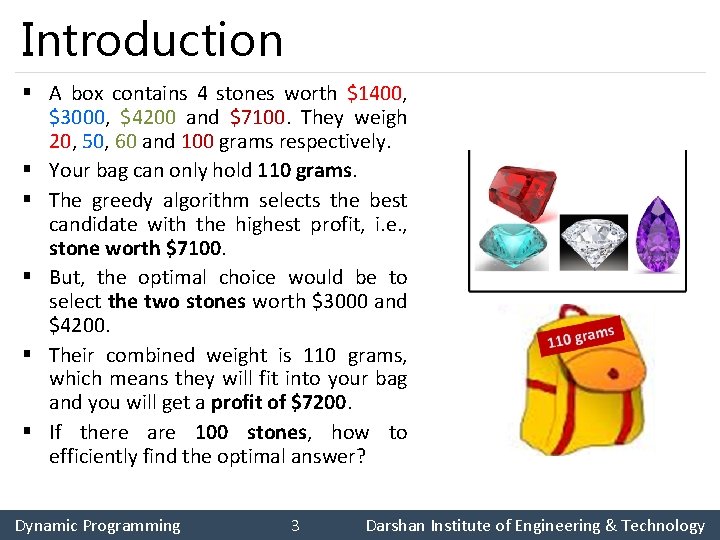
Introduction § A box contains 4 stones worth $1400, $3000, $4200 and $7100. They weigh 20, 50, 60 and 100 grams respectively. § Your bag can only hold 110 grams. § The greedy algorithm selects the best candidate with the highest profit, i. e. , stone worth $7100. § But, the optimal choice would be to select the two stones worth $3000 and $4200. § Their combined weight is 110 grams, which means they will fit into your bag and you will get a profit of $7200. § If there are 100 stones, how to efficiently find the optimal answer? Dynamic Programming 3 Darshan Institute of Engineering & Technology

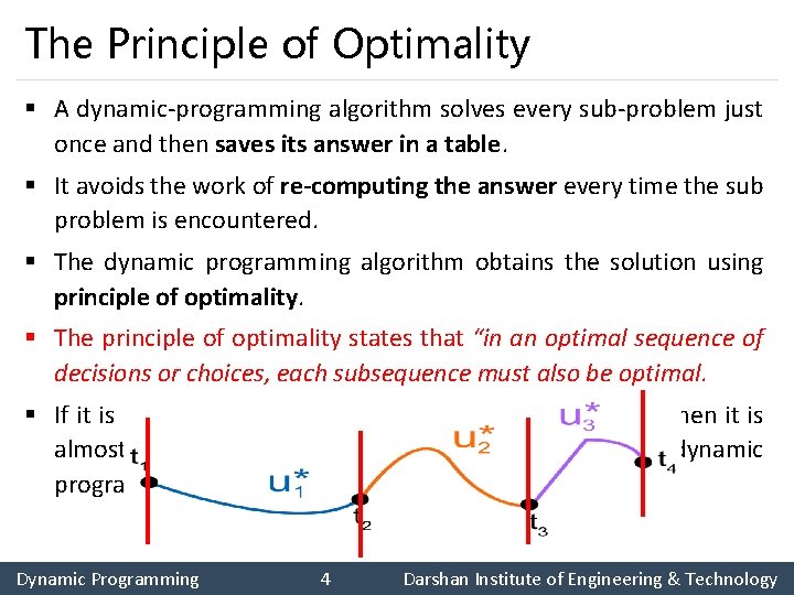
The Principle of Optimality § A dynamic-programming algorithm solves every sub-problem just once and then saves its answer in a table. § It avoids the work of re-computing the answer every time the sub problem is encountered. § The dynamic programming algorithm obtains the solution using principle of optimality. § The principle of optimality states that “in an optimal sequence of decisions or choices, each subsequence must also be optimal. § If it is not possible to apply the principle of optimality then it is almost impossible to obtain the solution using the dynamic programming approach. Dynamic Programming 4 Darshan Institute of Engineering & Technology

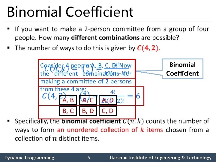
Binomial Coefficient § Consider 4 people A, B, C, D. Now the different combinations for making a committee of 2 persons from these 4 are; A, B B, C A, C B, D Binomial Coefficient A, D C, D Dynamic Programming 5 Darshan Institute of Engineering & Technology

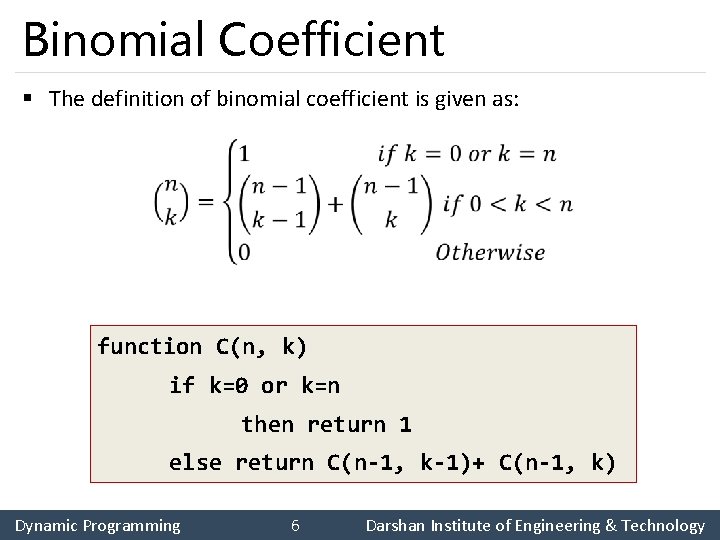
Binomial Coefficient § The definition of binomial coefficient is given as: function C(n, k) if k=0 or k=n then return 1 else return C(n-1, k-1)+ C(n-1, k) Dynamic Programming 6 Darshan Institute of Engineering & Technology

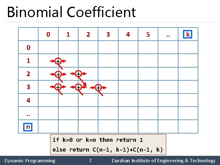
Binomial Coefficient 0 0 1 1 1 2 1 3 1 4 1 1 + + + 2 3 4 5 . . k 1 2 3 4 + + 1 3 6 + 1 4 1 . . n if k=0 or k=n then return 1 else return C(n-1, k-1)+C(n-1, k) Dynamic Programming 7 Darshan Institute of Engineering & Technology

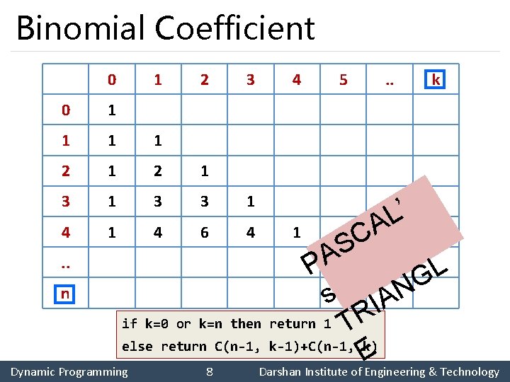
Binomial Coefficient 0 1 2 0 1 1 2 1 3 1 3 3 3 4 1 5 . . ’ L A k C S A. . P L G n s IAN if k=0 or k=n then return 1 TR else return C(n-1, k-1)+C(n-1, k) E Dynamic Programming 8 Darshan Institute of Engineering & Technology 4 1 4 6 4 1

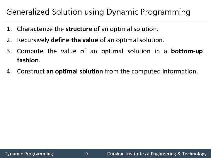
Generalized Solution using Dynamic Programming 1. Characterize the structure of an optimal solution. 2. Recursively define the value of an optimal solution. 3. Compute the value of an optimal solution in a bottom-up fashion. 4. Construct an optimal solution from the computed information. Dynamic Programming 9 Darshan Institute of Engineering & Technology

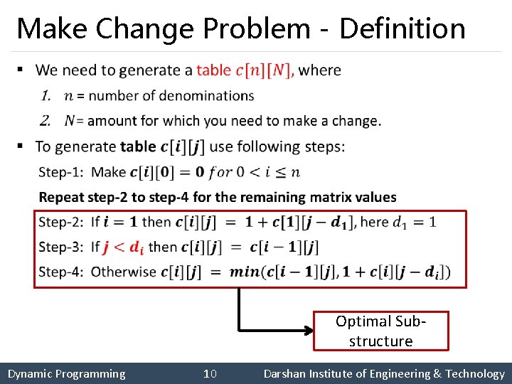
Make Change Problem - Definition § Optimal Substructure Dynamic Programming 10 Darshan Institute of Engineering & Technology

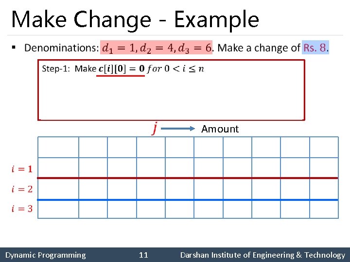
Make Change - Example § Amount 0 1 2 3 4 5 6 7 8 0 1 2 3 4 2 0 1 2 3 1 2 2 Dynamic Programming 11 Darshan Institute of Engineering & Technology

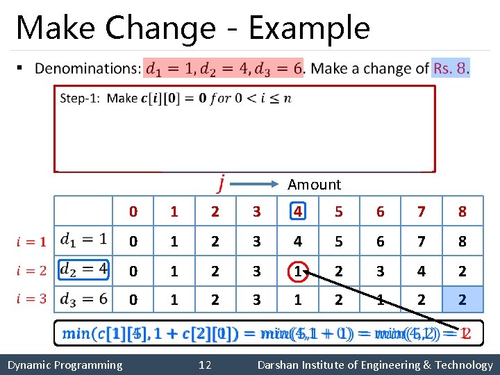
Make Change - Example § Amount 0 1 2 3 4 5 6 7 8 0 1 2 3 4 2 0 1 2 3 1 2 2 Dynamic Programming 12 Darshan Institute of Engineering & Technology

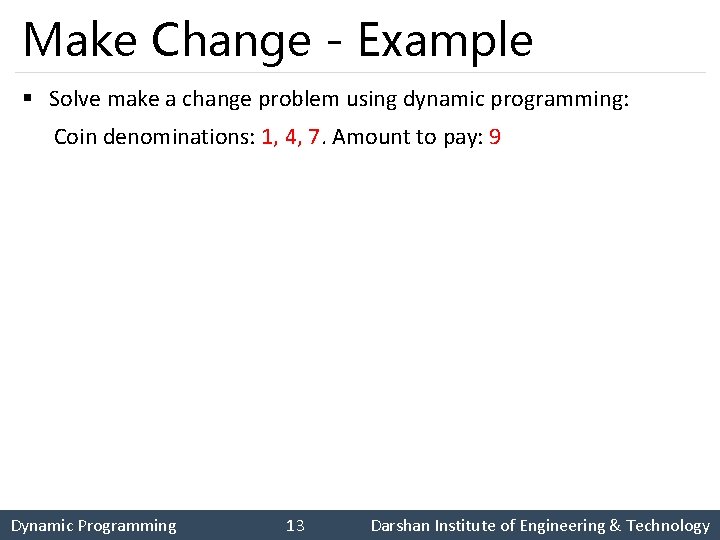
Make Change - Example § Solve make a change problem using dynamic programming: Coin denominations: 1, 4, 7. Amount to pay: 9 Dynamic Programming 13 Darshan Institute of Engineering & Technology

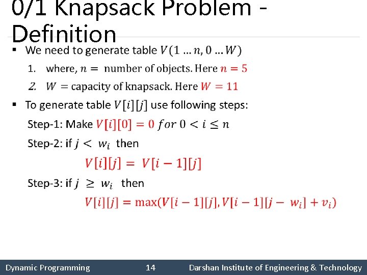
0/1 Knapsack Problem Definition § Dynamic Programming 14 Darshan Institute of Engineering & Technology

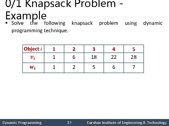
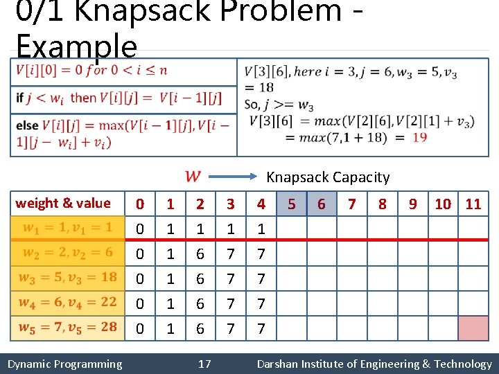
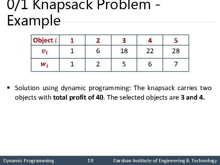
0/1 Knapsack Problem Example § Solve the following knapsack problem using dynamic programming technique. 1 1 2 6 3 18 4 22 5 28 1 2 5 6 7 Dynamic Programming 15 Darshan Institute of Engineering & Technology

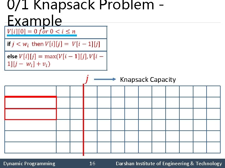
0/1 Knapsack Problem Example weight & value Knapsack Capacity 0 0 1 1 2 1 6 6 3 1 7 7 4 1 7 7 0 0 1 1 6 6 7 7 5 6 7 8 9 10 11 Dynamic Programming 16 Darshan Institute of Engineering & Technology

0/1 Knapsack Problem Example weight & value Knapsack Capacity 0 0 1 1 2 1 6 6 3 1 7 7 4 1 7 7 5 6 7 8 9 10 11 1 1 1 7 7 7 7 18 19 24 25 25 0 0 1 1 6 6 7 7 18 22 24 28 29 29 40 18 22 28 29 34 35 40 Dynamic Programming 17 Darshan Institute of Engineering & Technology

0/1 Knapsack Problem Example 1 1 2 6 3 18 4 22 5 28 1 2 5 6 7 § Solution using dynamic programming: The knapsack carries two objects with total profit of 40. The selected objects are 3 and 4. Dynamic Programming 18 Darshan Institute of Engineering & Technology

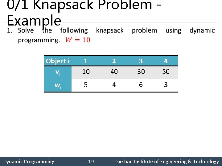
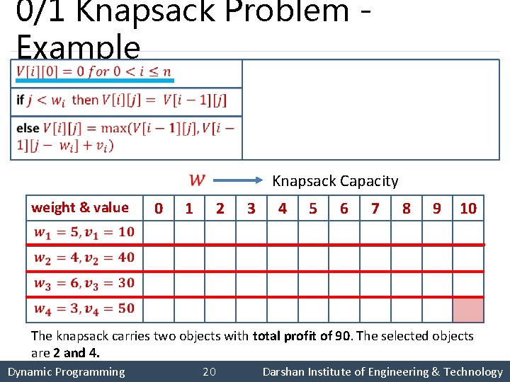
0/1 Knapsack Problem Example § Object i vi 1 10 2 40 3 30 4 50 wi 5 4 6 3 Dynamic Programming 19 Darshan Institute of Engineering & Technology

0/1 Knapsack Problem Example weight & value Knapsack Capacity 0 0 1 0 0 0 2 0 0 0 3 0 0 0 4 5 6 7 8 9 10 0 10 10 10 40 40 40 50 50 40 40 40 50 70 0 50 50 90 90 The knapsack carries two objects with total profit of 90. The selected objects are 2 and 4. Dynamic Programming 20 Darshan Institute of Engineering & Technology

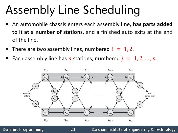
Assembly Line Scheduling § Dynamic Programming 21 Darshan Institute of Engineering & Technology

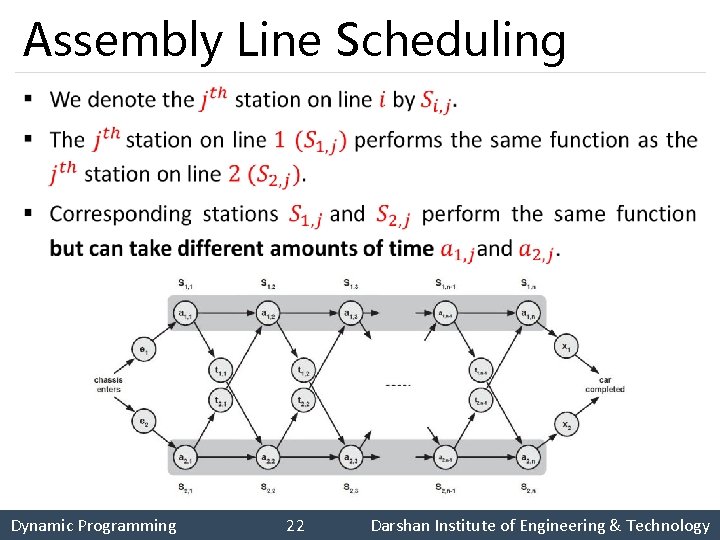
Assembly Line Scheduling § Dynamic Programming 22 Darshan Institute of Engineering & Technology

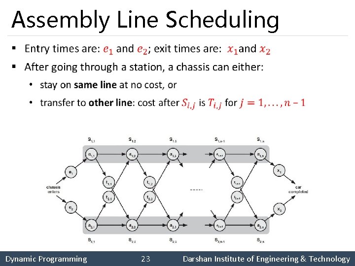
Assembly Line Scheduling § Dynamic Programming 23 Darshan Institute of Engineering & Technology

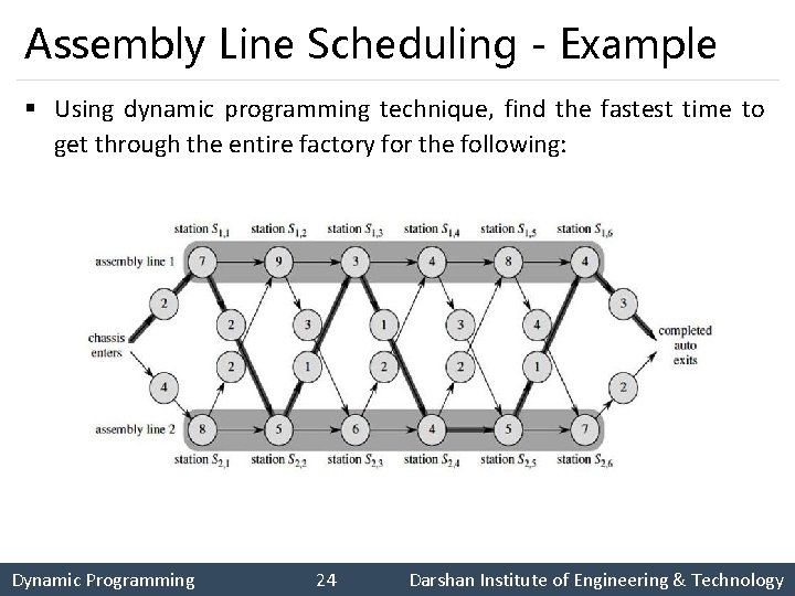
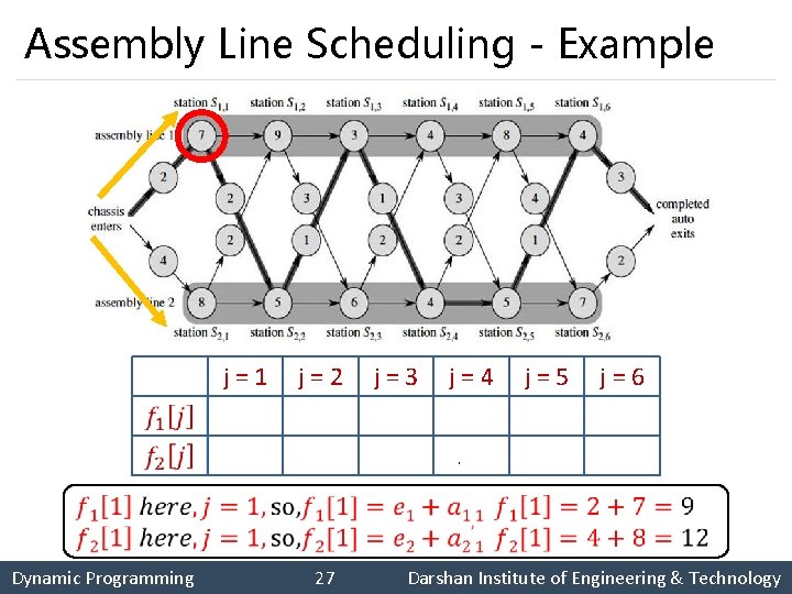
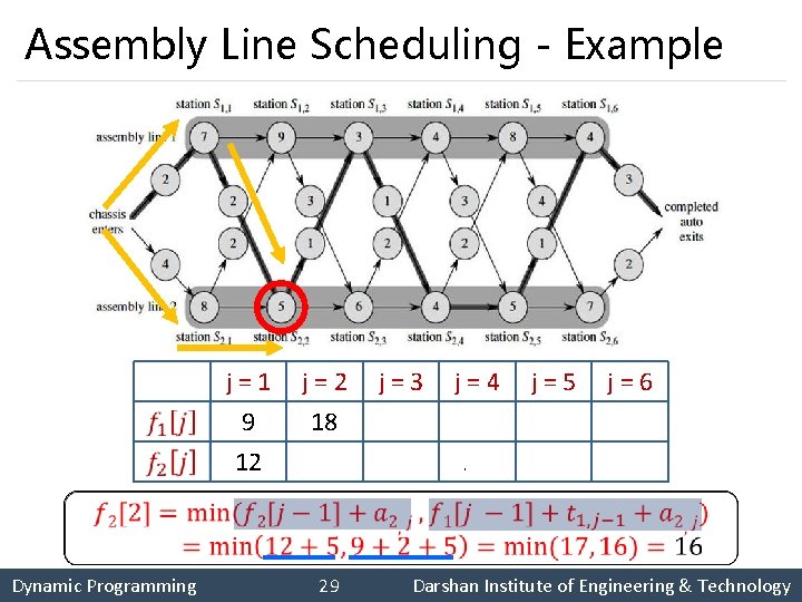
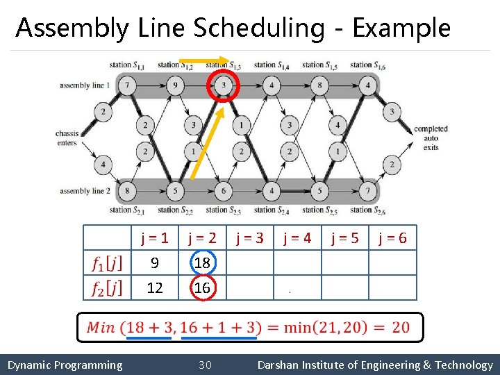
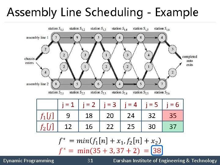
Assembly Line Scheduling - Example § Using dynamic programming technique, find the fastest time to get through the entire factory for the following: Dynamic Programming 24 Darshan Institute of Engineering & Technology

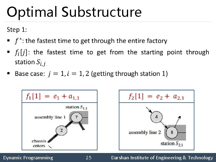
Optimal Substructure § Dynamic Programming 25 Darshan Institute of Engineering & Technology

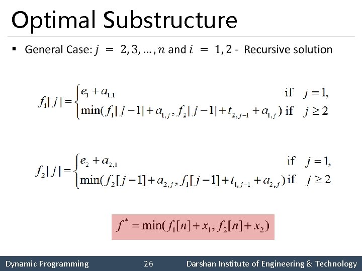
Optimal Substructure § Dynamic Programming 26 Darshan Institute of Engineering & Technology

Assembly Line Scheduling - Example j = 1 9 12 j = 2 18 16 j = 3 20 22 j = 4 24 25 j = 5 32 30 j = 6 35 37 Dynamic Programming 27 Darshan Institute of Engineering & Technology

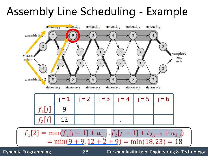
Assembly Line Scheduling - Example j = 1 9 12 j = 2 18 16 j = 3 20 22 j = 4 24 25 j = 5 32 30 j = 6 35 37 Dynamic Programming 28 Darshan Institute of Engineering & Technology

Assembly Line Scheduling - Example j = 1 9 12 j = 2 18 16 j = 3 20 22 j = 4 24 25 j = 5 32 30 j = 6 35 37 Dynamic Programming 29 Darshan Institute of Engineering & Technology

Assembly Line Scheduling - Example j = 1 9 12 j = 2 18 16 j = 3 20 22 j = 4 24 25 j = 5 32 30 j = 6 35 37 Dynamic Programming 30 Darshan Institute of Engineering & Technology

Assembly Line Scheduling - Example j = 1 9 12 j = 2 18 16 j = 3 20 22 j = 4 24 25 j = 5 32 30 j = 6 35 37 Dynamic Programming 31 Darshan Institute of Engineering & Technology

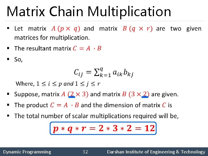
Matrix Chain Multiplication § Dynamic Programming 32 Darshan Institute of Engineering & Technology

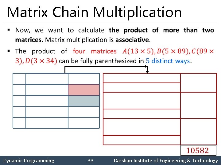
Matrix Chain Multiplication § 1 2 3 4 5 Dynamic Programming 33 Darshan Institute of Engineering & Technology

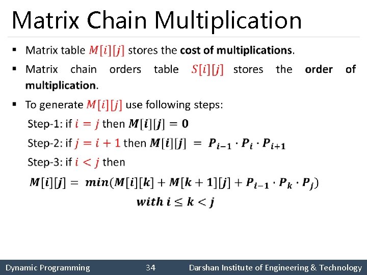
Matrix Chain Multiplication § Dynamic Programming 34 Darshan Institute of Engineering & Technology

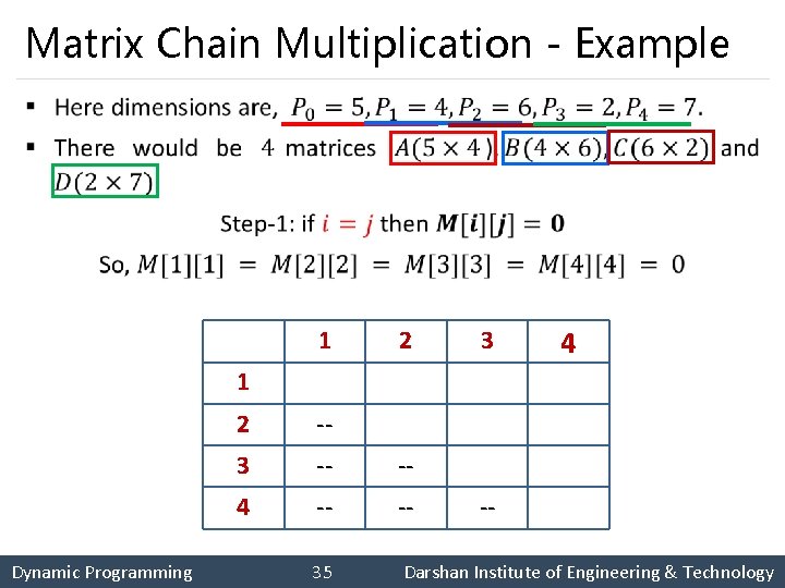
Matrix Chain Multiplication - Example § 1 2 3 1 0 2 -- 0 3 -- -- 0 4 -- -- -- 4 0 Dynamic Programming 35 Darshan Institute of Engineering & Technology

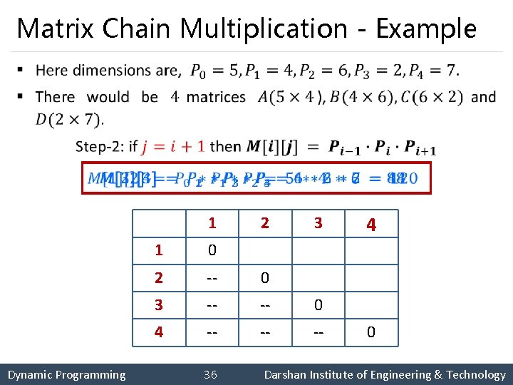
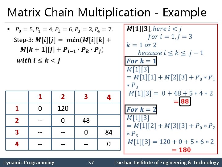
Matrix Chain Multiplication - Example § 1 2 3 1 0 120 2 -- 0 48 3 -- -- 0 84 4 -- -- -- 0 4 Dynamic Programming 36 Darshan Institute of Engineering & Technology

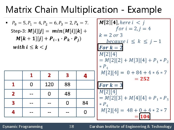
Matrix Chain Multiplication - Example § 1 2 3 1 0 120 88 2 -- 0 48 3 -- -- 0 84 4 -- -- -- 0 4 Dynamic Programming 37 Darshan Institute of Engineering & Technology

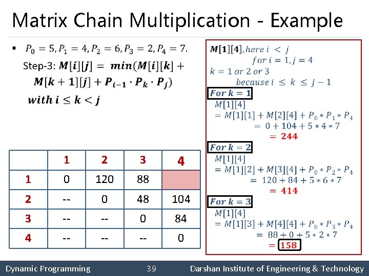
Matrix Chain Multiplication - Example § 1 2 3 1 0 120 88 2 -- 0 48 104 3 -- -- 0 84 4 -- -- -- 0 4 Dynamic Programming 38 Darshan Institute of Engineering & Technology

Matrix Chain Multiplication - Example § 1 2 3 4 1 0 120 88 158 2 -- 0 48 104 3 -- -- 0 84 4 -- -- -- 0 Dynamic Programming 39 Darshan Institute of Engineering & Technology

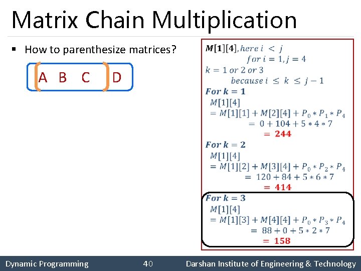
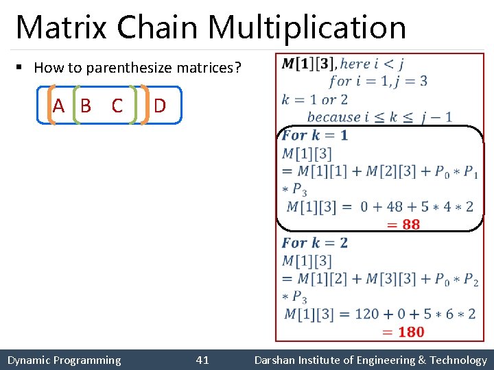
Matrix Chain Multiplication § How to parenthesize matrices? A B C D Dynamic Programming 40 Darshan Institute of Engineering & Technology

Matrix Chain Multiplication § How to parenthesize matrices? A B C D Dynamic Programming 41 Darshan Institute of Engineering & Technology

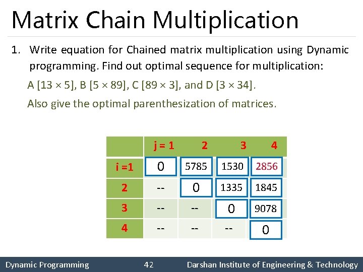
Matrix Chain Multiplication 1. Write equation for Chained matrix multiplication using Dynamic programming. Find out optimal sequence for multiplication: A [13 × 5], B [5 × 89], C [89 × 3], and D [3 × 34]. Also give the optimal parenthesization of matrices. j=1 2 3 4 i =1 0 5785 1530 2856 2 -- 0 1335 1845 3 -- -- 0 9078 4 -- -- -- 0 Dynamic Programming 42 Darshan Institute of Engineering & Technology

Matrix Chain Multiplication § How to parenthesize matrices? A B C D § M[1][4] k = 3 is selected minimum value. § M[1][3] k = 1 is selected minimum value. 1. ((AB)C)D 10582 2. (AB)(CD) 54201 3. (A(BC))D j=1 2 3 4 i= 0 5785 1530 2856 2 -- 0 1335 1845 4. A((BC)D) 4055 3 -- -- 0 9078 5. A(B(CD)) 26418 4 -- -- -- 0 Dynamic Programming 43 Darshan Institute of Engineering & Technology

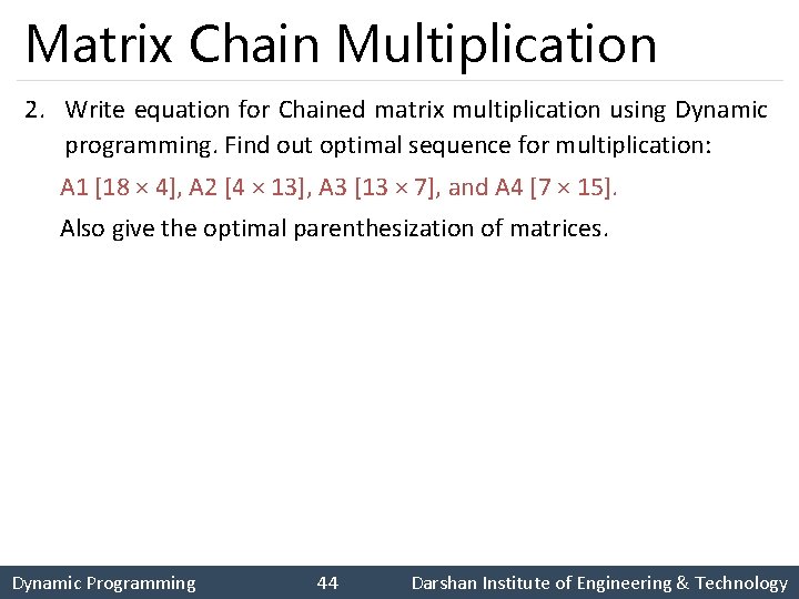
Matrix Chain Multiplication 2. Write equation for Chained matrix multiplication using Dynamic programming. Find out optimal sequence for multiplication: A 1 [18 × 4], A 2 [4 × 13], A 3 [13 × 7], and A 4 [7 × 15]. Also give the optimal parenthesization of matrices. Dynamic Programming 44 Darshan Institute of Engineering & Technology

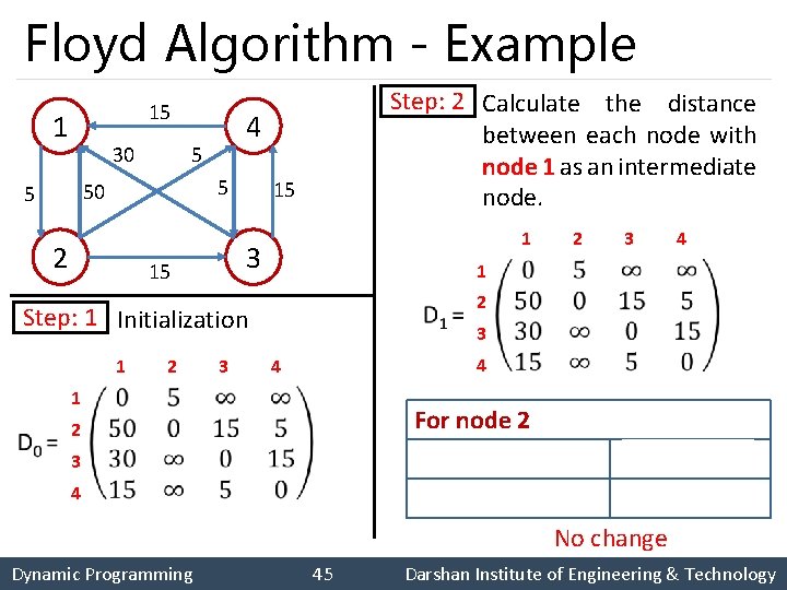
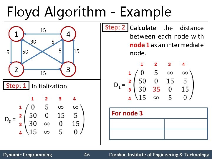
Floyd Algorithm - Example 15 1 30 5 5 50 5 4 2 15 3 15 1 1 2 2 3 1 2 3 4 1 2 Step: 1 Initialization Step: 2 Calculate the distance between each node with node 1 as an intermediate node. 3 4 4 For node 2 3 4 No change Dynamic Programming 45 Darshan Institute of Engineering & Technology

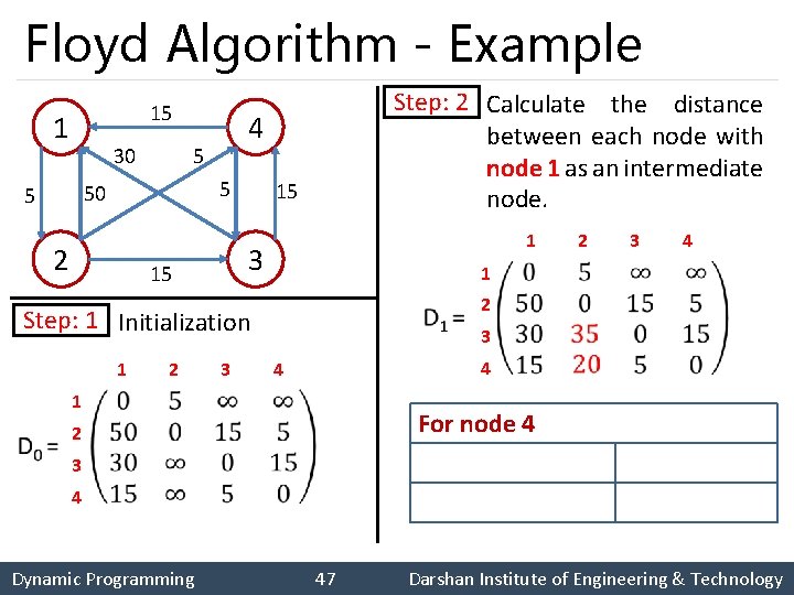
Floyd Algorithm - Example 15 1 30 5 5 50 5 4 2 15 3 15 1 1 2 2 3 1 2 3 4 1 2 Step: 1 Initialization Step: 2 Calculate the distance between each node with node 1 as an intermediate node. 3 4 4 For node 3 3 4 Dynamic Programming 46 Darshan Institute of Engineering & Technology

Floyd Algorithm - Example 15 1 30 5 5 50 5 4 2 15 3 15 1 2 2 3 1 2 3 4 1 2 Step: 1 Initialization 1 Step: 2 Calculate the distance between each node with node 1 as an intermediate node. 3 4 4 For node 4 3 4 Dynamic Programming 47 Darshan Institute of Engineering & Technology

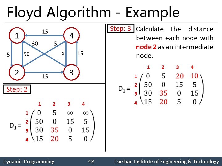
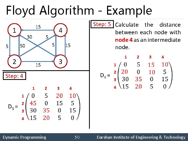
Floyd Algorithm - Example 15 1 30 5 5 50 5 4 2 15 3 15 1 1 2 3 4 2 Step: 2 Step: 3 Calculate the distance between each node with node 2 as an intermediate node. 3 1 2 3 4 4 1 2 3 4 Dynamic Programming 48 Darshan Institute of Engineering & Technology

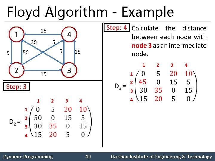
Floyd Algorithm - Example 15 1 30 5 5 50 5 4 2 15 3 15 1 2 3 4 1 2 Step: 3 Step: 4 Calculate the distance between each node with node 3 as an intermediate node. 3 1 2 3 4 4 1 2 3 4 Dynamic Programming 49 Darshan Institute of Engineering & Technology

Floyd Algorithm - Example 15 1 30 5 5 50 5 4 2 15 3 15 1 2 3 4 1 2 Step: 4 Step: 5 Calculate the distance between each node with node 4 as an intermediate node. 3 1 2 3 4 4 1 2 3 4 Dynamic Programming 50 Darshan Institute of Engineering & Technology

Floyd’s Algorithm function Floyd(L[1. . n, 1. . n]): array [1. . n, 1. . n] array D[1. . n, 1. . n] D ← L for k ← 1 to n do for i ← 1 to n do for j ← 1 to n do D[i, j] ← min(D[i, j], D[i, k]+ D[k, j]) return Dn temp ← A[j] A[j+1] ← temp Dynamic Programming 51 Darshan Institute of Engineering & Technology

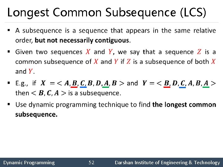
Longest Common Subsequence (LCS) § Dynamic Programming 52 Darshan Institute of Engineering & Technology

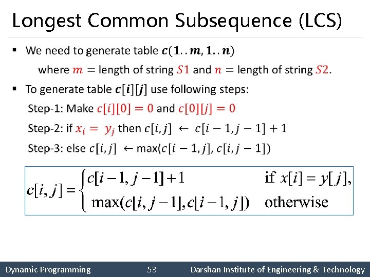
Longest Common Subsequence (LCS) § Dynamic Programming 53 Darshan Institute of Engineering & Technology

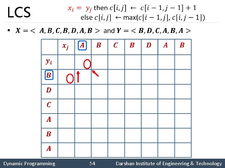
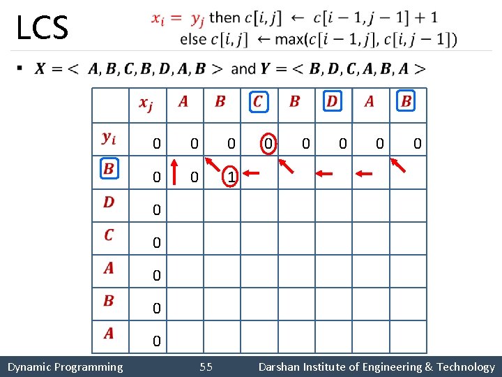
LCS § 0 0 0 0 0 1 1 1 2 2 2 0 0 1 2 2 2 0 1 1 2 2 2 3 3 0 1 2 2 3 3 3 4 0 1 2 2 3 3 4 4 Dynamic Programming 54 Darshan Institute of Engineering & Technology

LCS § 0 0 0 0 0 1 1 1 2 2 2 0 0 1 2 2 2 0 1 1 2 2 2 3 3 0 1 2 2 3 3 3 4 0 1 2 2 3 3 4 4 Dynamic Programming 55 Darshan Institute of Engineering & Technology

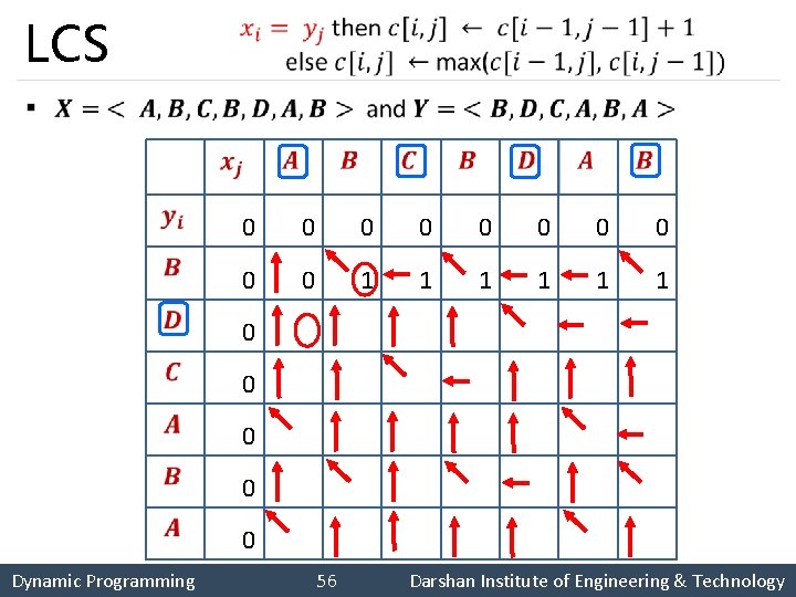
LCS § 0 0 0 0 0 1 1 1 2 2 2 0 0 1 2 2 2 0 1 1 2 2 2 3 3 0 1 2 2 3 3 3 4 0 1 2 2 3 3 4 4 Dynamic Programming 56 Darshan Institute of Engineering & Technology

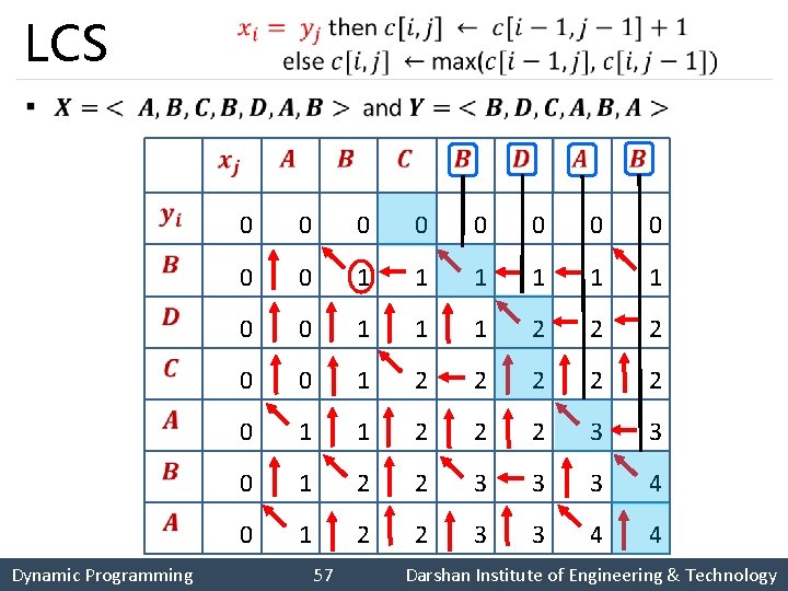
LCS § 0 0 0 0 0 1 1 1 2 2 2 0 0 1 2 2 2 0 1 1 2 2 2 3 3 0 1 2 2 3 3 3 4 0 1 2 2 3 3 4 4 Dynamic Programming 57 Darshan Institute of Engineering & Technology

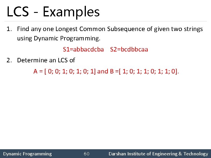
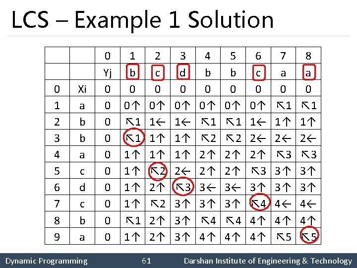
LCS - Examples 1. Find any one Longest Common Subsequence of given two strings using Dynamic Programming. S 1=abbacdcba S 2=bcdbbcaa 2. Determine an LCS of A = [ 0; 0; 1; 0; 1] and B =[ 1; 0; 1; 1; 0]. Dynamic Programming 60 Darshan Institute of Engineering & Technology

LCS – Example 1 Solution 0 1 2 3 4 5 6 7 8 9 Xi a b b a c d c b a 0 Yj 0 0 0 0 0 1 b 0 0↑ ↖ 1 1↑ 1↑ ↖ 1 1↑ 2 c 0 0↑ 1← 1↑ 1↑ ↖ 2 2↑ 2↑ 3 d 0 0↑ 1← 1↑ 1↑ 2← ↖ 3 3↑ 3↑ 3↑ 4 b 0 0↑ ↖ 1 ↖ 2 2↑ 2↑ 3← 3↑ ↖ 4 4↑ 5 b 0 0↑ ↖ 1 ↖ 2 2↑ 2↑ 3← 3↑ ↖ 4 4↑ 6 c 0 0↑ 1← 2← 2↑ ↖ 3 3↑ ↖ 4 4↑ 4↑ 7 a 0 ↖ 1 1↑ 2← ↖ 3 3↑ 3↑ 4← 4↑ ↖ 5 8 a 0 ↖ 1 1↑ 2← ↖ 3 3↑ 3↑ 4← 4↑ ↖ 5 Dynamic Programming 61 Darshan Institute of Engineering & Technology

Thank You Greedy Algorithm 62 Darshan Institute of Engineering & Technology