Unit 3 Nonlinear Data Structure Graph Prof Pradyumansinh

Unit – 3 Nonlinear Data Structure Graph Prof. Pradyumansinh Jadeja � 9879461848 �pradyuman. jadeja@darshan. ac. in Data Structure (2130702) Darshan Institute of Engineering & Technology

Graphs § What is Graph? § Representation of Graph • Matrix representation of Graph • Linked List representation of Graph § Elementary Graph Operations • Breadth First Search (BFS) • Depth First Search (DFS) • Spanning Trees • Minimal Spanning Trees • Shortest Path Unit – 3: Non Linear Data Structure Tree 2 Darshan Institute of Engineering & Technology

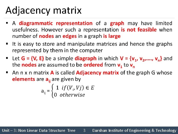
Adjacency matrix § Unit – 3: Non Linear Data Structure Tree 3 Darshan Institute of Engineering & Technology

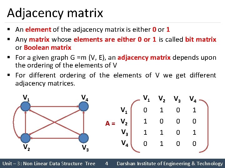
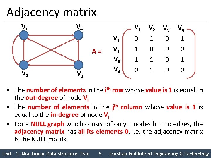
Adjacency matrix § An element of the adjacency matrix is either 0 or 1 § Any matrix whose elements are either 0 or 1 is called bit matrix or Boolean matrix § For a given graph G =m (V, E), an adjacency matrix depends upon the ordering of the elements of V § For different ordering of the elements of V we get different adjacency matrices. V 1 V 4 V 1 V 2 V 3 Unit – 3: Non Linear Data Structure Tree A = V 2 V 3 V 4 4 V 1 V 2 V 3 V 4 0 1 1 0 0 1 0 Darshan Institute of Engineering & Technology

Adjacency matrix V 1 V 4 V 1 A= V 2 V 3 V 4 V 1 V 2 V 3 V 4 0 1 1 0 0 1 0 § The number of elements in the ith row whose value is 1 is equal to the out-degree of node Vi § The number of elements in the jth column whose value is 1 is equal to the in-degree of node Vj § For a NULL graph which consist of only n nodes but no edges, the adjacency matrix has all its elements 0. i. e. the adjacency matrix is the NULL matrix Unit – 3: Non Linear Data Structure Tree 5 Darshan Institute of Engineering & Technology

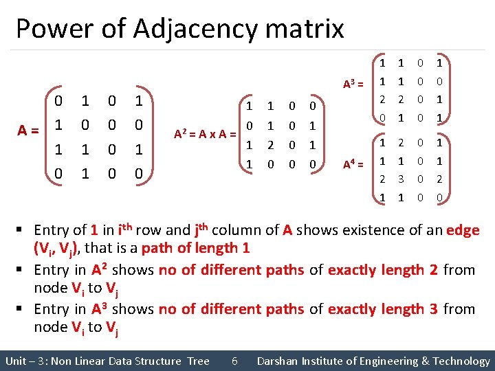
Power of Adjacency matrix 0 A= 1 1 0 0 1 0 1 0 A 2 = A x A = 1 1 2 0 0 0 1 1 0 A 3 = 1 1 2 0 1 1 2 1 0 0 1 0 1 1 A 4 = 1 1 2 1 3 1 0 0 1 1 2 0 § Entry of 1 in ith row and jth column of A shows existence of an edge (Vi, Vj), that is a path of length 1 § Entry in A 2 shows no of different paths of exactly length 2 from node Vi to Vj § Entry in A 3 shows no of different paths of exactly length 3 from node Vi to Vj Unit – 3: Non Linear Data Structure Tree 6 Darshan Institute of Engineering & Technology

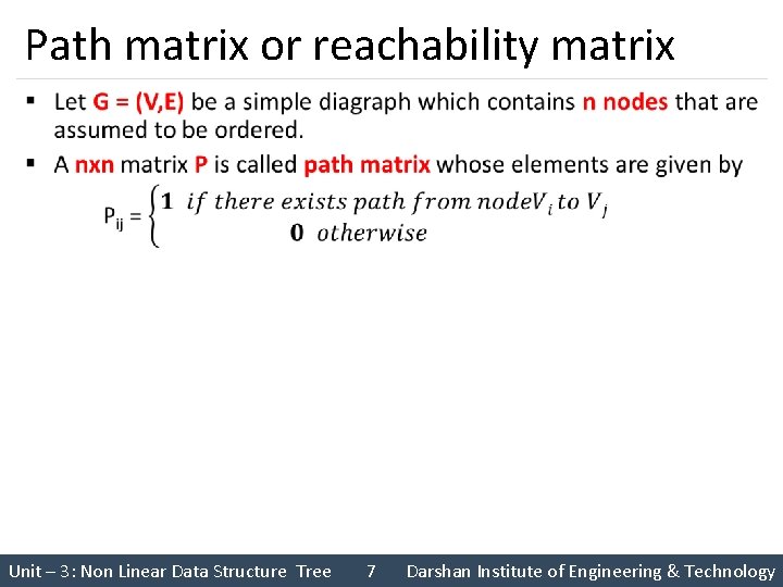
Path matrix or reachability matrix § Unit – 3: Non Linear Data Structure Tree 7 Darshan Institute of Engineering & Technology

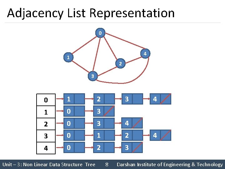
Adjacency List Representation 0 4 1 2 3 0 1 2 1 0 3 2 0 3 4 3 0 1 2 4 0 2 3 Unit – 3: Non Linear Data Structure Tree 3 8 4 4 Darshan Institute of Engineering & Technology

Graph Traversal § Two Commonly used Traversal Techniques are • Depth First Search (DFS) • Breadth First Search (BFS) Unit – 3: Non Linear Data Structure Tree 9 Darshan Institute of Engineering & Technology

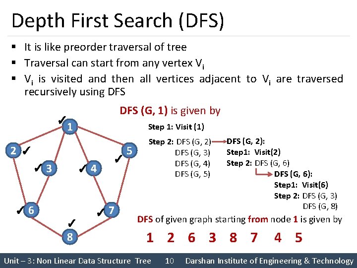
Depth First Search (DFS) § It is like preorder traversal of tree § Traversal can start from any vertex Vi § Vi is visited and then all vertices adjacent to Vi are traversed recursively using DFS (G, 1) is given by ✓ 1 Step 1: Visit (1) 2 ✓ ✓ 3 ✓ 4 ✓ 6 ✓ ✓ 7 ✓ 8 5 Step 2: DFS (G, 2) DFS (G, 3) DFS (G, 4) DFS (G, 5) DFS (G, 2): Step 1: Visit(2) Step 2: DFS (G, 6): Step 1: Visit(6) Step 2: DFS (G, 3) DFS (G, 8) DFS of given graph starting from node 1 is given by 1 2 6 3 8 7 Unit – 3: Non Linear Data Structure Tree 10 4 5 Darshan Institute of Engineering & Technology

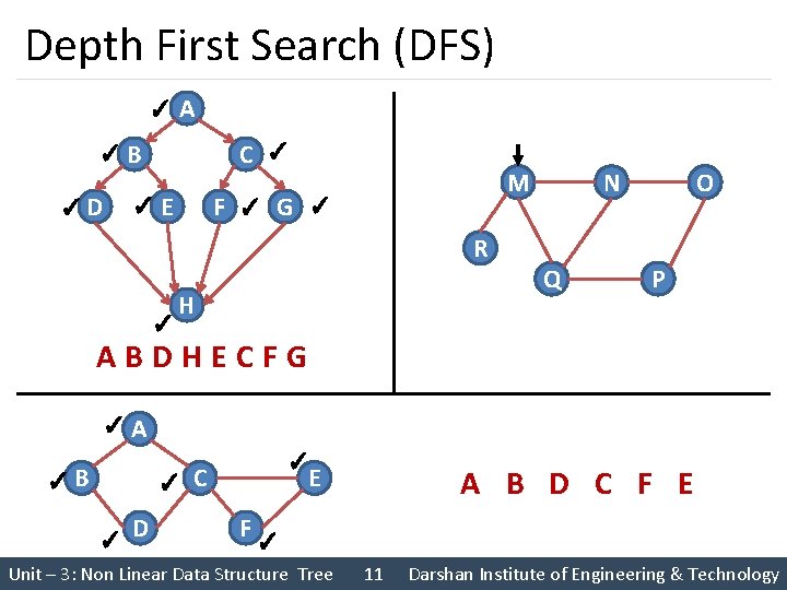
Depth First Search (DFS) ✓ A ✓B ✓D C ✓ ✓E M F ✓ G ✓ R ✓ H O N Q P ABDHECFG ✓A ✓B ✓ ✓ D ✓ C E A B D C F E F✓ Unit – 3: Non Linear Data Structure Tree 11 Darshan Institute of Engineering & Technology

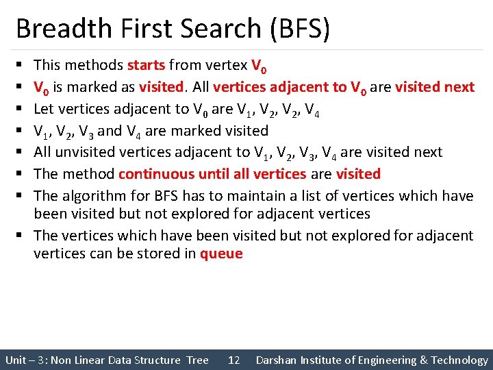
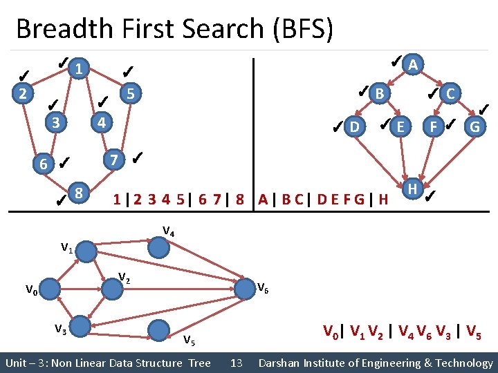
Breadth First Search (BFS) This methods starts from vertex V 0 is marked as visited. All vertices adjacent to V 0 are visited next Let vertices adjacent to V 0 are V 1, V 2, V 4 V 1, V 2, V 3 and V 4 are marked visited All unvisited vertices adjacent to V 1, V 2, V 3, V 4 are visited next The method continuous until all vertices are visited The algorithm for BFS has to maintain a list of vertices which have been visited but not explored for adjacent vertices § The vertices which have been visited but not explored for adjacent vertices can be stored in queue § § § § Unit – 3: Non Linear Data Structure Tree 12 Darshan Institute of Engineering & Technology

Breadth First Search (BFS) ✓ 2 ✓ 1 ✓ ✓ 5 ✓ 4 ✓ 3 6 ✓ ✓ 8 ✓ ✓E F✓ G 1 | 2 3 4 5 | 6 7 | 8 A | B C| D E F G | H C ✓ H✓ V 4 V 2 V 3 B 7 ✓ V 1 V 0 D A V 6 V 0 | V 1 V 2 | V 4 V 6 V 3 | V 5 Unit – 3: Non Linear Data Structure Tree 13 Darshan Institute of Engineering & Technology

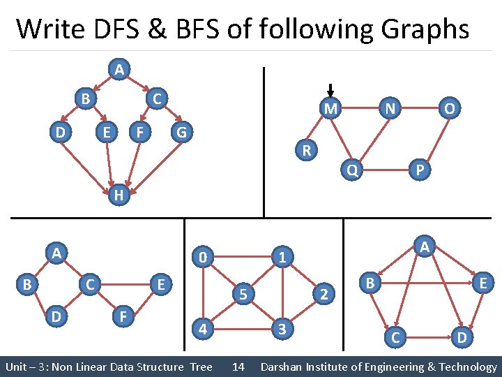
Write DFS & BFS of following Graphs A B D C E F M G R O N Q P H A B 0 C D E F 5 4 Unit – 3: Non Linear Data Structure Tree A 1 2 3 14 B E C D Darshan Institute of Engineering & Technology

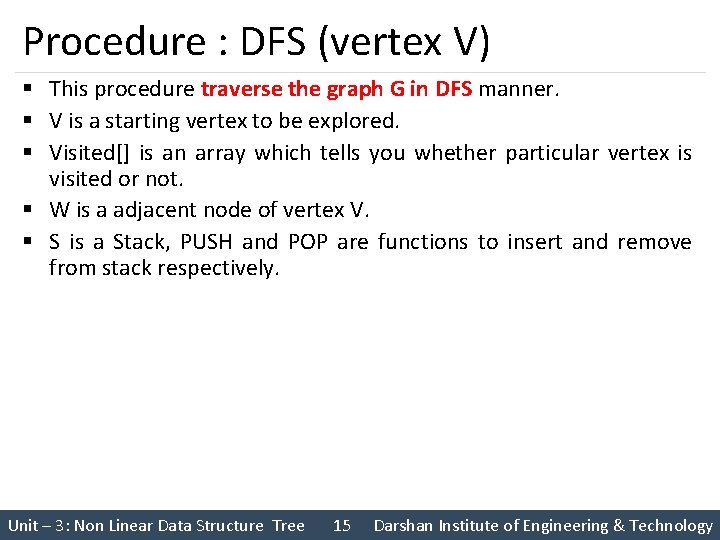
Procedure : DFS (vertex V) § This procedure traverse the graph G in DFS manner. § V is a starting vertex to be explored. § Visited[] is an array which tells you whether particular vertex is visited or not. § W is a adjacent node of vertex V. § S is a Stack, PUSH and POP are functions to insert and remove from stack respectively. Unit – 3: Non Linear Data Structure Tree 15 Darshan Institute of Engineering & Technology

Procedure : DFS (vertex V) 1. [Initialize TOP and Visited] visited[] 0 TOP 0 2. [Push vertex into stack] PUSH (V) 3. [Repeat while stack is not Empty] Repeat step 3 while stack is not empty v POP() if visited[v] is 0 then visited [v] 1 for all W adjacent to v if visited [w] is 0 then PUSH (W) end for end if Unit – 3: Non Linear Data Structure Tree 16 Darshan Institute of Engineering & Technology

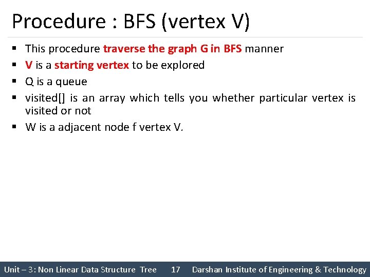
Procedure : BFS (vertex V) This procedure traverse the graph G in BFS manner V is a starting vertex to be explored Q is a queue visited[] is an array which tells you whether particular vertex is visited or not § W is a adjacent node f vertex V. § § Unit – 3: Non Linear Data Structure Tree 17 Darshan Institute of Engineering & Technology

Procedure : BFS (vertex V) 1. [Initialize Queue & Visited] visited[] 0 F R 0 2. [Marks visited of V as 1] visited[v] 1 3. [Add vertex v to Q] Insert. Queue(V) 4. [Repeat while Q is not Empty] Repeat while Q is not empty v Remove. From. Queue() For all vertices W adjacent to v if visited[w] is 0 then visited[w] 1 Insert. Queue(w) Unit – 3: Non Linear Data Structure Tree 18 Darshan Institute of Engineering & Technology

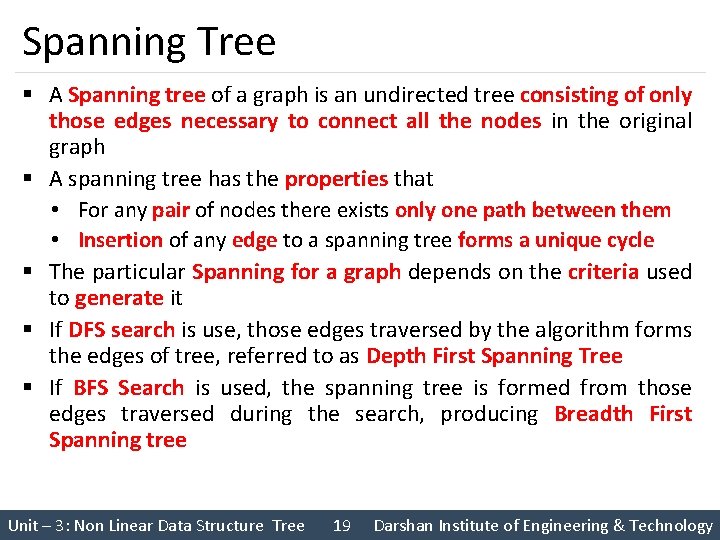
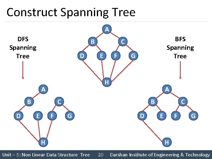
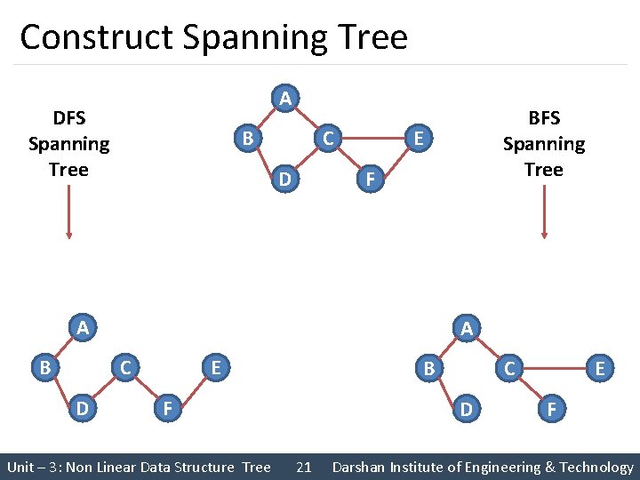
Spanning Tree § A Spanning tree of a graph is an undirected tree consisting of only those edges necessary to connect all the nodes in the original graph § A spanning tree has the properties that • For any pair of nodes there exists only one path between them • Insertion of any edge to a spanning tree forms a unique cycle § The particular Spanning for a graph depends on the criteria used to generate it § If DFS search is use, those edges traversed by the algorithm forms the edges of tree, referred to as Depth First Spanning Tree § If BFS Search is used, the spanning tree is formed from those edges traversed during the search, producing Breadth First Spanning tree Unit – 3: Non Linear Data Structure Tree 19 Darshan Institute of Engineering & Technology

Construct Spanning Tree A DFS Spanning Tree B D E F G H A B D BFS Spanning Tree C A C E F B G D H Unit – 3: Non Linear Data Structure Tree C E F G H 20 Darshan Institute of Engineering & Technology

Construct Spanning Tree A DFS Spanning Tree B C D E F A B A C D BFS Spanning Tree E B F Unit – 3: Non Linear Data Structure Tree C D 21 E F Darshan Institute of Engineering & Technology

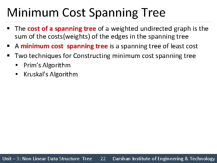
Minimum Cost Spanning Tree § The cost of a spanning tree of a weighted undirected graph is the sum of the costs(weights) of the edges in the spanning tree § A minimum cost spanning tree is a spanning tree of least cost § Two techniques for Constructing minimum cost spanning tree • Prim’s Algorithm • Kruskal’s Algorithm Unit – 3: Non Linear Data Structure Tree 22 Darshan Institute of Engineering & Technology

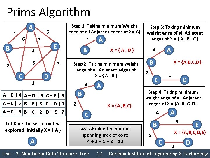
Prims Algorithm A 4 6 6 B 5 5 C 1 4 E 3 2 Step 1: Taking minimum Weight edge of all Adjacent edges of X={A} B 7 D A–B|4 A–D|6 C–E|5 A–E|5 B–E|3 C–D|1 A–C|6 B–C|2 D–E|7 Let X be the set of nodes explored, initially X = { A } A A B A 2 X = {A , B, C} B 2 X = {A, B, C, D} C 4 We obtained minimum spanning tree of cost: 4 + 2 + 1 + 3 = 10 23 1 D Step 4: Taking minimum weight edge of all Adjacent edges of X = {A , B , C , D } C Unit – 3: Non Linear Data Structure Tree A 4 X={A, B} Step 2: Taking minimum weight edge of all Adjacent edges of X={A, B} 4 Step 3: Taking minimum weight edge of all Adjacent edges of X = { A , B , C } 3 B 2 A E X = {A, B, C, D, E} C D 1 Darshan Institute of Engineering & Technology

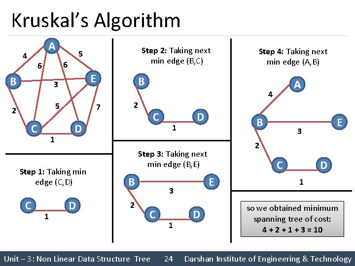
Kruskal’s Algorithm A 4 6 6 B E 3 5 2 C 1 1 2 C 1 D B B C Unit – 3: Non Linear Data Structure Tree 1 24 D 3 C E 3 E 2 Step 3: Taking next min edge (B, E) 2 A 4 D D Step 4: Taking next min edge (A, B) B 7 Step 1: Taking min edge (C, D) C Step 2: Taking next min edge (B, C) 5 D 1 so we obtained minimum spanning tree of cost: 4 + 2 + 1 + 3 = 10 Darshan Institute of Engineering & Technology

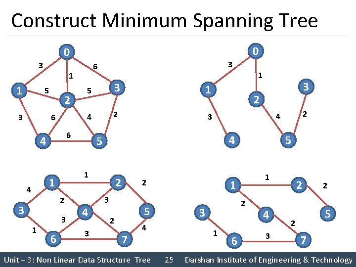
Construct Minimum Spanning Tree 0 0 3 1 1 5 3 2 6 2 3 1 4 2 3 3 6 4 3 1 3 2 4 2 2 3 2 7 1 2 3 4 Unit – 3: Non Linear Data Structure Tree 5 1 25 2 4 5 1 1 4 5 6 4 3 6 6 4 3 2 2 5 2 7 Darshan Institute of Engineering & Technology

Shortest Path Algorithm § Let G = (V, E) be a simple diagraph with n vertices § The problem is to find out shortest distance from a vertex to all other vertices of a graph § Dijkstra Algorithm – it is also called Single Source Shortest Path Algorithm Unit – 3: Non Linear Data Structure Tree 26 Darshan Institute of Engineering & Technology

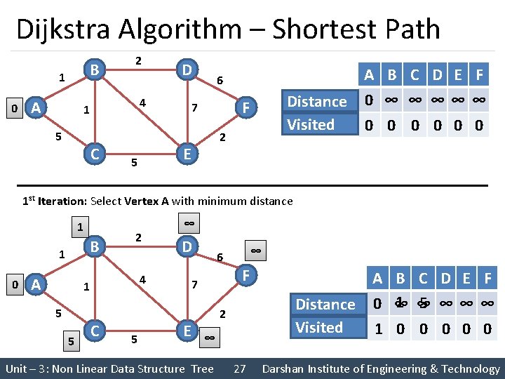
Dijkstra Algorithm – Shortest Path B 1 0 A 2 4 1 5 D C 6 2 E 5 Distance Visited F 7 A B C D E F 0 ∞ ∞ ∞∞ ∞ 0 0 0 1 st Iteration: Select Vertex A with minimum distance 1 B 1 0 A 2 5 D 4 1 5 ∞ C 5 F 7 E ∞ 6 Distance Visited 2 ∞ Unit – 3: Non Linear Data Structure Tree 27 A 0 1 B C D E F 1 ∞ 5 ∞∞ ∞ ∞ 0 0 0 Darshan Institute of Engineering & Technology

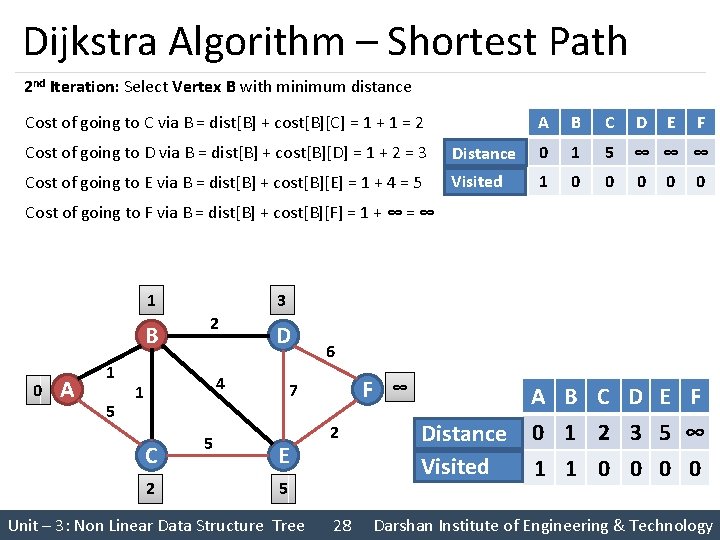
Dijkstra Algorithm – Shortest Path 2 nd Iteration: Select Vertex B with minimum distance Cost of going to C via B = dist[B] + cost[B][C] = 1 + 1 = 2 A B C D E F Cost of going to D via B = dist[B] + cost[B][D] = 1 + 2 = 3 Distance 0 1 5 ∞ ∞ ∞ Cost of going to E via B = dist[B] + cost[B][E] = 1 + 4 = 5 Visited 1 0 0 0 Cost of going to F via B = dist[B] + cost[B][F] = 1 + ∞ = ∞ 3 1 B 0 A 1 5 2 D 4 1 C 2 5 6 F 7 E 2 5 Unit – 3: Non Linear Data Structure Tree 28 ∞ Distance Visited A B C D E F 0 1 2 3 5 ∞ 1 1 0 0 Darshan Institute of Engineering & Technology

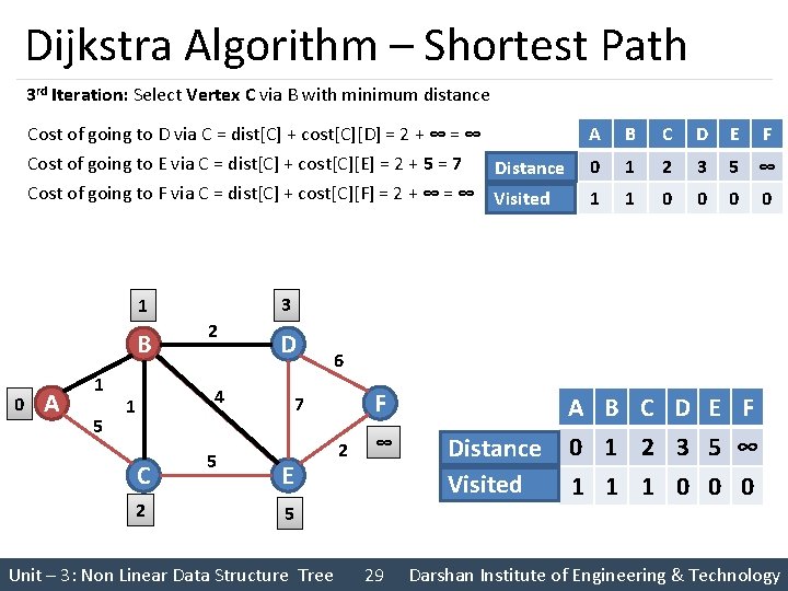
Dijkstra Algorithm – Shortest Path 3 rd Iteration: Select Vertex C via B with minimum distance Cost of going to D via C = dist[C] + cost[C][D] = 2 + ∞ = ∞ Cost of going to E via C = dist[C] + cost[C][E] = 2 + 5 = 7 Distance Cost of going to F via C = dist[C] + cost[C][F] = 2 + ∞ = ∞ Visited 0 A 1 5 2 D 4 1 C 2 B C D E F 0 1 2 3 5 ∞ 1 1 0 0 3 1 B A 5 6 F 7 E 2 ∞ 5 Unit – 3: Non Linear Data Structure Tree 29 Distance Visited A B C D E F 0 1 2 3 5 ∞ 1 1 1 0 0 0 Darshan Institute of Engineering & Technology

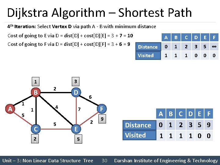
Dijkstra Algorithm – Shortest Path 4 th Iteration: Select Vertex D via path A - B with minimum distance Cost of going to E via D = dist[D] + cost[D][E] = 3 + 7 = 10 Cost of going to F via D = dist[D] + cost[D][F] = 3 + 6 = 9 A 1 5 2 D 4 1 C 2 B C D E F Distance 0 1 2 3 5 ∞ Visited 1 1 1 0 0 0 3 1 B A 5 6 F 7 E 2 9 5 Unit – 3: Non Linear Data Structure Tree 30 Distance Visited A B C D E F 0 1 2 3 5 9 1 1 0 0 Darshan Institute of Engineering & Technology

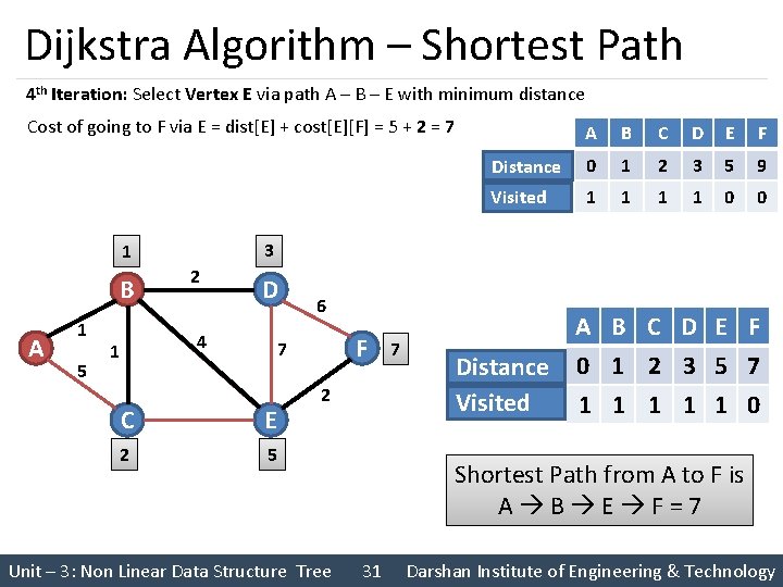
Dijkstra Algorithm – Shortest Path 4 th Iteration: Select Vertex E via path A – B – E with minimum distance Cost of going to F via E = dist[E] + cost[E][F] = 5 + 2 = 7 A 1 5 2 D 4 1 B C D E F Distance 0 1 2 3 5 9 Visited 1 1 0 0 3 1 B A 6 F 7 C E 2 5 2 Unit – 3: Non Linear Data Structure Tree 7 Distance Visited A B C D E F 0 1 2 3 5 7 1 1 1 0 Shortest Path from A to F is A B E F=7 31 Darshan Institute of Engineering & Technology

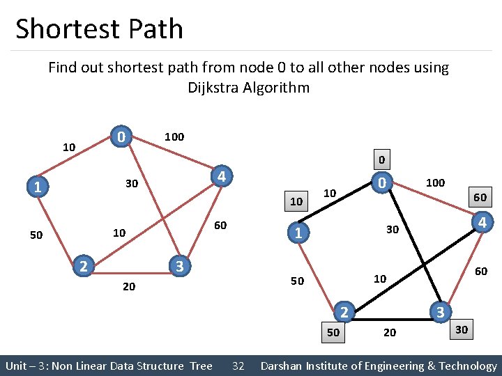
Shortest Path Find out shortest path from node 0 to all other nodes using Dijkstra Algorithm 0 10 100 4 30 1 0 10 60 10 50 2 0 10 2 50 Unit – 3: Non Linear Data Structure Tree 32 4 60 10 50 20 60 30 1 3 100 3 20 30 Darshan Institute of Engineering & Technology