Unit 3 Monetary Policy Keynesian Models ISLM 4192011

Unit 3: Monetary Policy Keynesian Models (ISLM) 4/19/2011

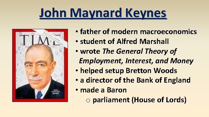
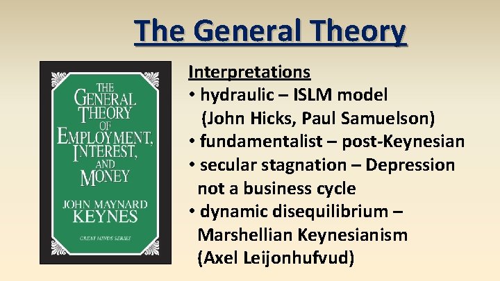
John Maynard Keynes • father of modern macroeconomics • student of Alfred Marshall • wrote The General Theory of Employment, Interest, and Money • helped setup Bretton Woods • a director of the Bank of England • made a Baron o parliament (House of Lords)

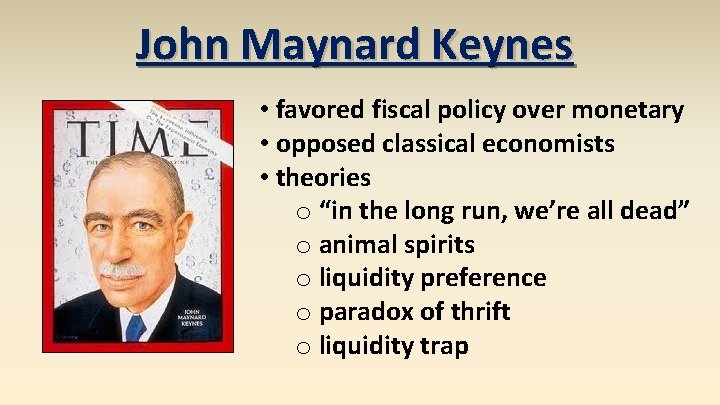
John Maynard Keynes • favored fiscal policy over monetary • opposed classical economists • theories o “in the long run, we’re all dead” o animal spirits o liquidity preference o paradox of thrift o liquidity trap

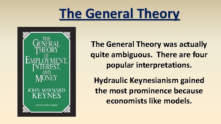
The General Theory was actually quite ambiguous. There are four popular interpretations. Hydraulic Keynesianism gained the most prominence because economists like models.

The General Theory Interpretations • hydraulic – ISLM model (John Hicks, Paul Samuelson) • fundamentalist – post-Keynesian • secular stagnation – Depression not a business cycle • dynamic disequilibrium – Marshellian Keynesianism (Axel Leijonhufvud)

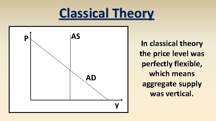
Classical Theory P AS In classical theory the price level was perfectly flexible, which means aggregate supply was vertical. AD y

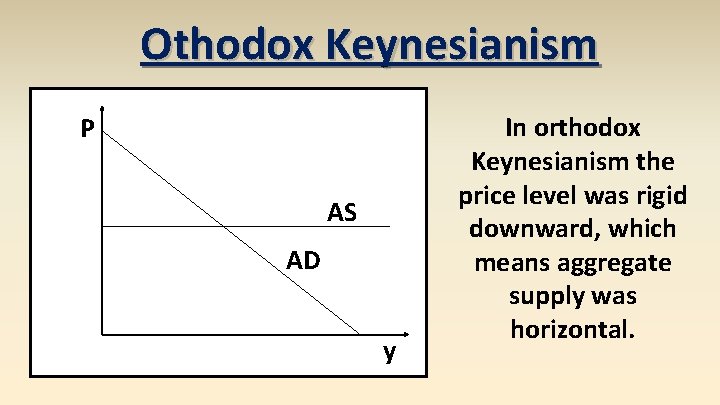
Othodox Keynesianism P AS AD y In orthodox Keynesianism the price level was rigid downward, which means aggregate supply was horizontal.

Keynes vs. Classicals Classical economists believed the price level would adjust whenever aggregate demand shifted, so government interventions could have no effect on aggregate output. Keynes believed classical economics held in the long run, but in the short run the price level wouldn’t adjust.

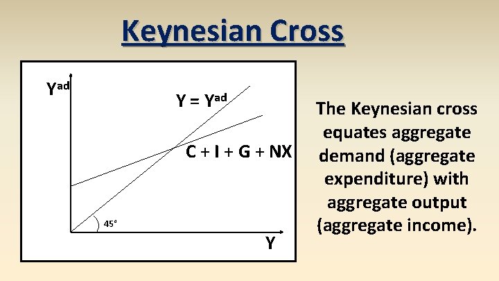
Keynesian Cross Yad Y = Yad C + I + G + NX 45° Y The Keynesian cross equates aggregate demand (aggregate expenditure) with aggregate output (aggregate income).

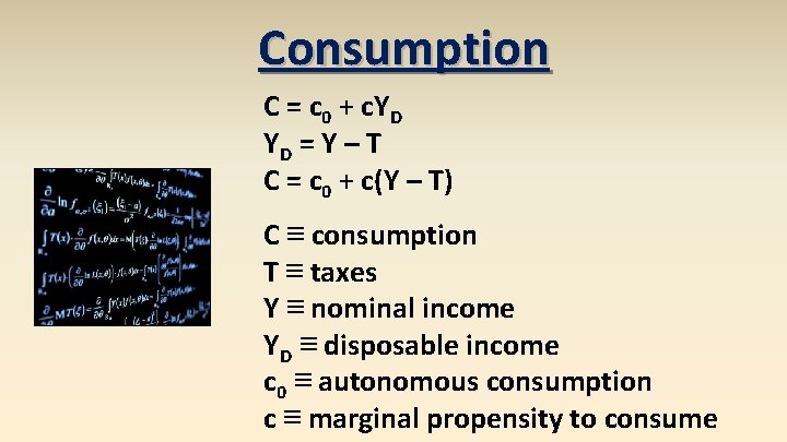
Consumption C = c 0 + c. YD YD = Y – T C = c 0 + c(Y – T) C ≡ consumption T ≡ taxes Y ≡ nominal income YD ≡ disposable income c 0 ≡ autonomous consumption c ≡ marginal propensity to consume

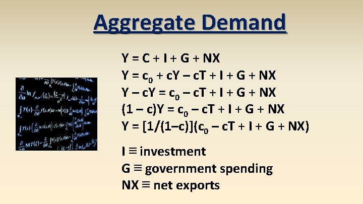
Aggregate Demand Y = C + I + G + NX Y = c 0 + c. Y – c. T + I + G + NX Y – c. Y = c 0 – c. T + I + G + NX (1 – c)Y = c 0 – c. T + I + G + NX Y = [1/(1–c)](c 0 – c. T + I + G + NX) I ≡ investment G ≡ government spending NX ≡ net exports

Aggregate Demand Increases in consumption, investment, government spending, net exports, and autonomous consumption are positively related to an increase in output. An increase in taxes is negatively related to an increase in output.

Investment Note that economists use the word “investment” different from ordinary people. Investment is the purchase of new physical assets (e. g. , new machines or new houses). Used assets don’t count, nor do common stocks or bonds.

Animal Spirits animal spirits – emotional waves of optimism and pessimism that influence investment spending, causing wild fluctuations Keynes believed changes in spending were dominated by investment spending, unstable due to “animal spirits. ”

Keynesian Multipliers Y = C + I + G + NX Y = [1/(1–c)](c 0 – c. T + I + G + NX) Multipliers • ΔY/ΔI = 1/(1–c) • ΔY/ΔG = 1/(1–c) • ΔY/ΔNX = 1/(1–c) • ΔY/Δc 0 = 1/(1–c) • ΔY/ΔT = -c/(1–c)

Keynesian Multipliers The tax multiplier is less than the other multipliers. It is multiplied by the marginal propensity to consume (c), which is less than 1. This leads Keynesians to believe that increases in government spending are more effective than tax cuts.

Critique of Keynesianism Comparing spending to tax multipliers doesn’t take into account the growth incentives of low taxes. Aggregation obscures that some spending is less useful than other spending. (e. g. , Frederic Bastiat’s broken window fallacy)

Broken Window Fallacy Some economists suggested that government spending increases output because of a multiplier: if government builds a bridge, the bridge workers buy bread, then bakers buy shoes, etc.

Broken Window Fallacy Bastiat pointed out by that logic you should break a window (or break every window in France), because then the homeowner would pay repairmen to fix the window, the repairmen buys bread, then bakers buy shoes, etc.

Broken Window Fallacy But if the money had not been spent repairing the window, it would have been spent on something else with a similar multiplier. The broken window is “what is seen, ” whereas the alternative purchase is “what is unseen” (the opportunity cost).

Broken Window Fallacy So breaking windows doesn’t really help the economy. Nor does wasting money on useless public projects such as digging ditches – the lost multiplier is collected taxes that could have been spent by consumers.

Broken Window Fallacy broken window fallacy – fallacy of taking into account easy to see positive effects of a policy, but not taking into account negative hidden effects of a policy

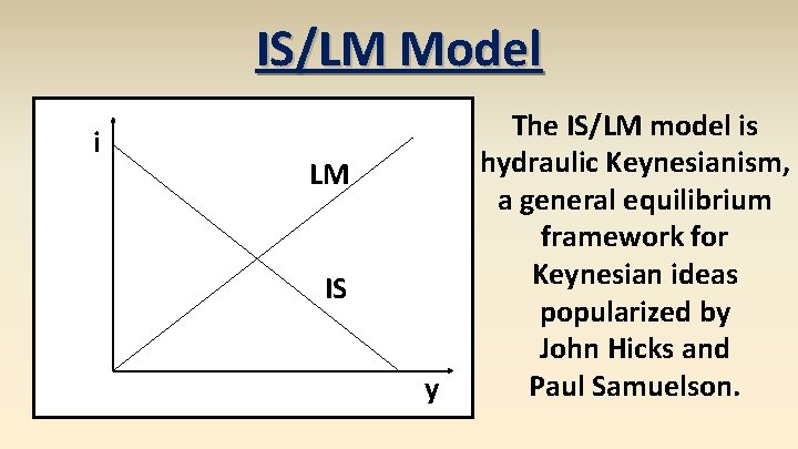
IS/LM Model i LM IS y The IS/LM model is hydraulic Keynesianism, a general equilibrium framework for Keynesian ideas popularized by John Hicks and Paul Samuelson.

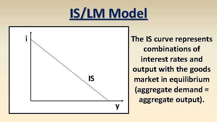
IS/LM Model i IS y The IS curve represents combinations of interest rates and output with the goods market in equilibrium (aggregate demand = aggregate output).

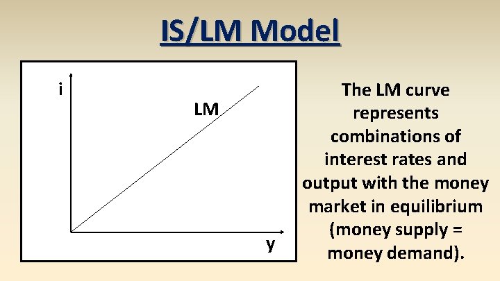
IS/LM Model i LM y The LM curve represents combinations of interest rates and output with the money market in equilibrium (money supply = money demand).

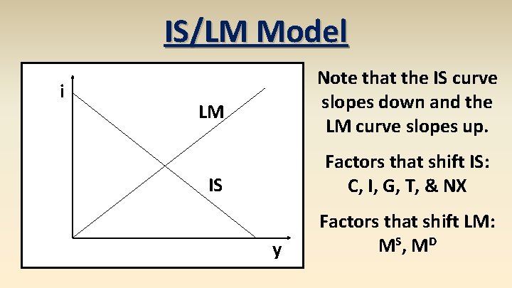
IS/LM Model i Note that the IS curve slopes down and the LM curve slopes up. LM Factors that shift IS: C, I, G, T, & NX IS y Factors that shift LM: MS , M D

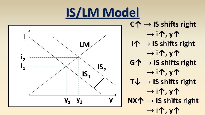
IS/LM Model i i 2 i 1 LM IS 1 y 2 IS 2 y C↑ → IS shifts right → i↑, y↑ I↑ → IS shifts right → i↑, y↑ G↑ → IS shifts right → i↑, y↑ T↓ → IS shifts right → i↑, y↑ NX↑ → IS shifts right → i↑, y↑

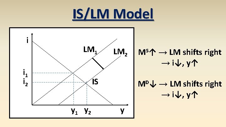
IS/LM Model i LM 1 i 2 LM 2 IS y 1 y 2 MS↑ → LM shifts right → i↓, y↑ MD↓ → LM shifts right → i↓, y↑ y

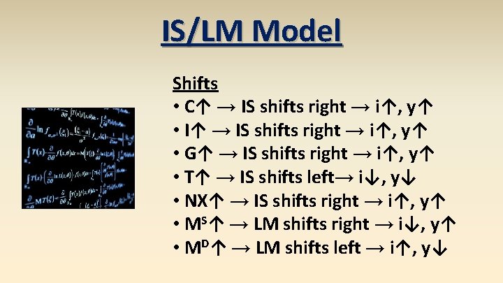
IS/LM Model Shifts • C↑ → IS shifts right → i↑, y↑ • I↑ → IS shifts right → i↑, y↑ • G↑ → IS shifts right → i↑, y↑ • T↑ → IS shifts left→ i↓, y↓ • NX↑ → IS shifts right → i↑, y↑ • MS↑ → LM shifts right → i↓, y↑ • MD↑ → LM shifts left → i↑, y↓

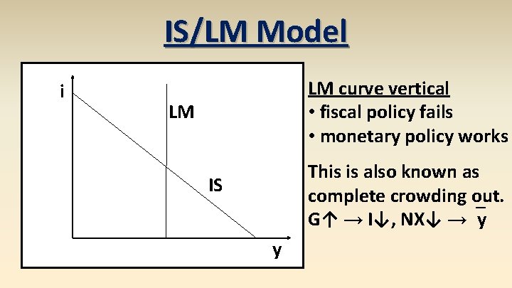
IS/LM Model i LM curve vertical • fiscal policy fails • monetary policy works LM This is also known as complete crowding out. G↑ → I↓, NX↓ →`y IS y

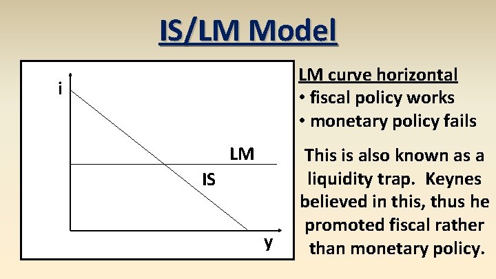
IS/LM Model LM curve horizontal • fiscal policy works • monetary policy fails i LM IS y This is also known as a liquidity trap. Keynes believed in this, thus he promoted fiscal rather than monetary policy.

Liquidity Trap liquidity trap – demand for money is infinitely elastic (LM curve horizontal), causing monetary policy to be completely ineffective Neoclassical economists refute this through the Pigou Effect: real money balances influence consumption and the IS curve.

Critique of Keynesianism Keynes recommended that governments run deficits (fiscal stimulus) during recessions and surpluses (fiscal dampener) during booms. Politicians heard economists say “sometimes run deficits” and forgot the “sometimes” part.

Critique of Keynesianism Politicians use economists like drunks use lampposts: more for support than illumination.

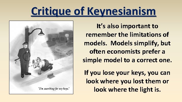
Critique of Keynesianism It’s also important to remember the limitations of models. Models simplify, but often economists prefer a simple model to a correct one. If you lose your keys, you can look where you lost them or look where the light is.

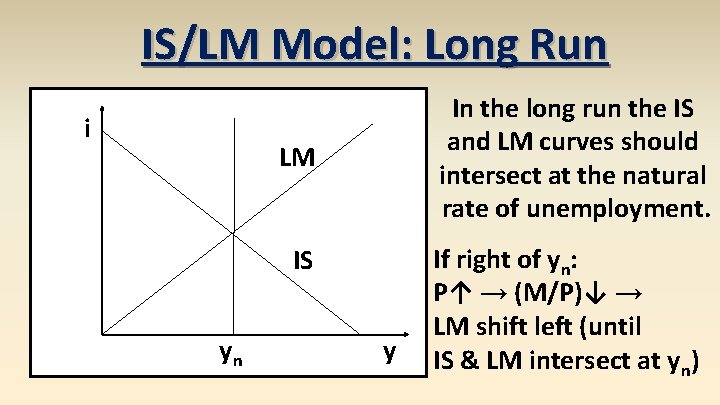
IS/LM Model: Long Run i In the long run the IS and LM curves should intersect at the natural rate of unemployment. LM IS yn y If right of yn: P↑ → (M/P)↓ → LM shift left (until IS & LM intersect at yn)

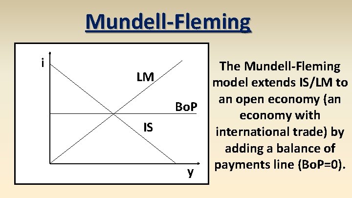
Mundell-Fleming i LM Bo. P IS y The Mundell-Fleming model extends IS/LM to an open economy (an economy with international trade) by adding a balance of payments line (Bo. P=0).

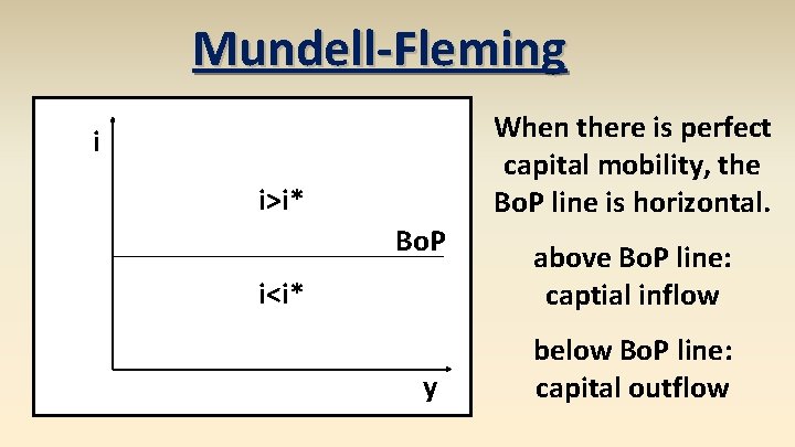
Mundell-Fleming When there is perfect capital mobility, the Bo. P line is horizontal. i i>i* Bo. P i<i* y above Bo. P line: captial inflow below Bo. P line: capital outflow

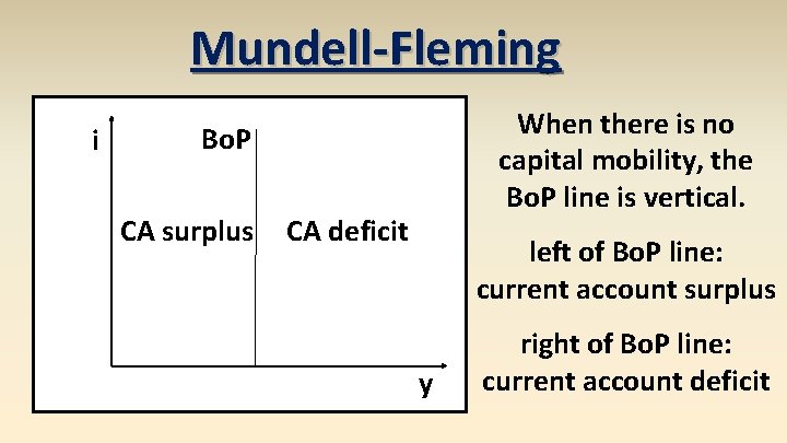
Mundell-Fleming i When there is no capital mobility, the Bo. P line is vertical. Bo. P CA surplus CA deficit left of Bo. P line: current account surplus y right of Bo. P line: current account deficit

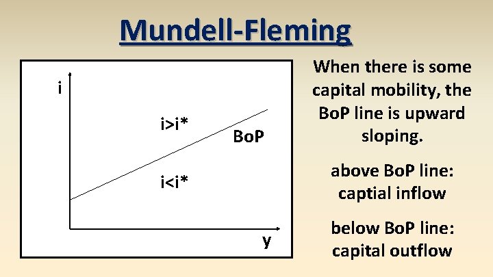
Mundell-Fleming i i>i* Bo. P When there is some capital mobility, the Bo. P line is upward sloping. above Bo. P line: captial inflow i<i* y below Bo. P line: capital outflow

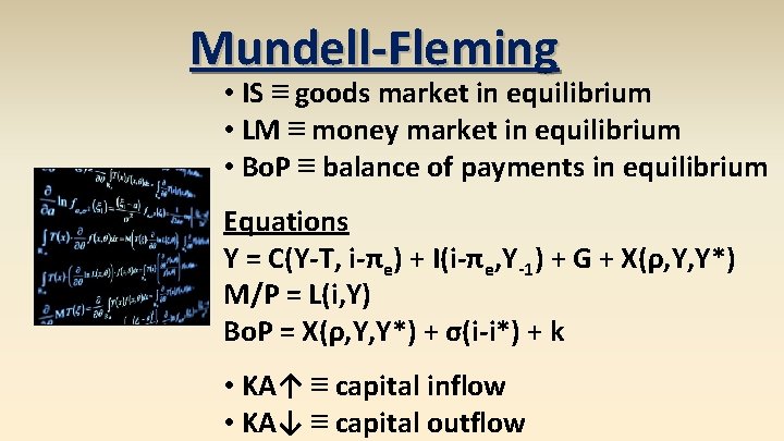
Mundell-Fleming • IS ≡ goods market in equilibrium • LM ≡ money market in equilibrium • Bo. P ≡ balance of payments in equilibrium Equations Y = C(Y-T, i-πe) + I(i-πe, Y-1) + G + X(ρ, Y, Y*) M/P = L(i, Y) Bo. P = X(ρ, Y, Y*) + σ(i-i*) + k • KA↑ ≡ capital inflow • KA↓ ≡ capital outflow

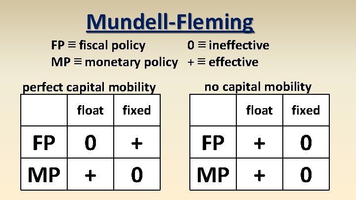
Mundell-Fleming FP ≡ fiscal policy 0 ≡ ineffective MP ≡ monetary policy + ≡ effective perfect capital mobility no capital mobility float fixed 0 + + 0 0 FP MP

Mundell-Fleming Figuring it out • float o IS + Bo. P curves move • fixed o LM curve moves • perfect/some capital mobility o mechanism: interest rates • no capital mobility o mechanism: goods trade

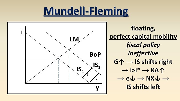
Mundell-Fleming i LM IS 1 Bo. P IS 2 1 2 y floating, perfect capital mobility fiscal policy ineffective G↑ → IS shifts right → i>i* → KA↑ → e↓ → NX↓ → IS shifts left

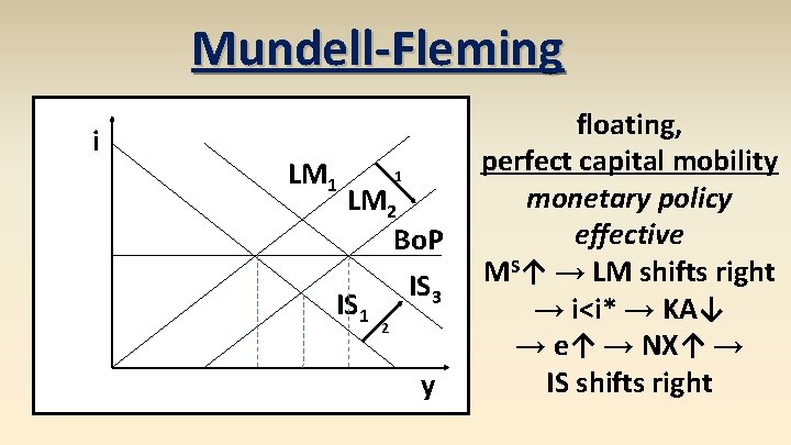
Mundell-Fleming i LM 1 1 LM 2 Bo. P IS 3 IS 1 2 y floating, perfect capital mobility monetary policy effective MS↑ → LM shifts right → i<i* → KA↓ → e↑ → NX↑ → IS shifts right

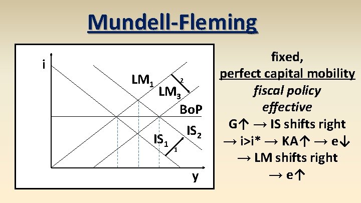
Mundell-Fleming i LM 1 2 LM 3 Bo. P IS 2 IS 1 1 y fixed, perfect capital mobility fiscal policy effective G↑ → IS shifts right → i>i* → KA↑ → e↓ → LM shifts right → e↑

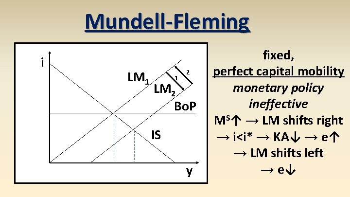
Mundell-Fleming i LM 1 1 2 LM 2 Bo. P IS y fixed, perfect capital mobility monetary policy ineffective MS↑ → LM shifts right → i<i* → KA↓ → e↑ → LM shifts left → e↓

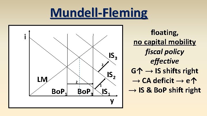
Mundell-Fleming i IS 3 2 LM 2 Bo. P 1 Bo. P 3 IS 2 1 IS 1 y floating, no capital mobility fiscal policy effective G↑ → IS shifts right → CA deficit → e↑ → IS & Bo. P shift right

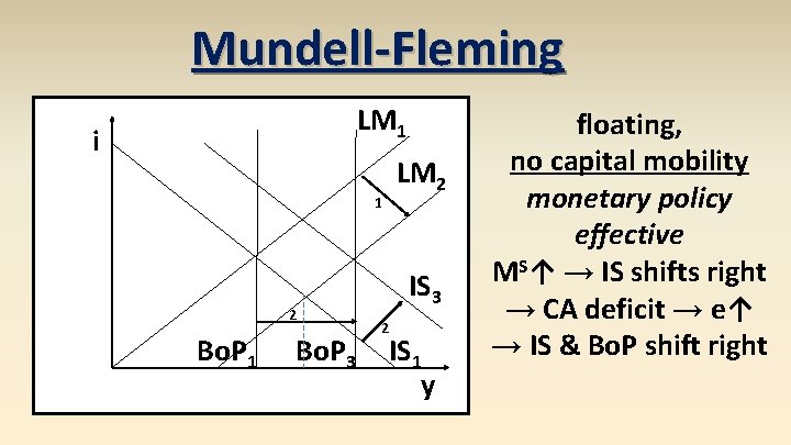
Mundell-Fleming LM 1 i LM 2 1 2 Bo. P 1 Bo. P 3 IS 3 2 IS 1 y floating, no capital mobility monetary policy effective MS↑ → IS shifts right → CA deficit → e↑ → IS & Bo. P shift right

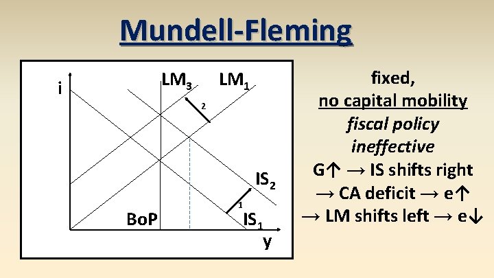
Mundell-Fleming LM 3 i LM 1 2 IS 2 Bo. P 1 IS 1 y fixed, no capital mobility fiscal policy ineffective G↑ → IS shifts right → CA deficit → e↑ → LM shifts left → e↓

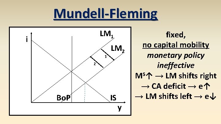
Mundell-Fleming LM 1 i 1 LM 2 2 Bo. P IS y fixed, no capital mobility monetary policy ineffective MS↑ → LM shifts right → CA deficit → e↑ → LM shifts left → e↓

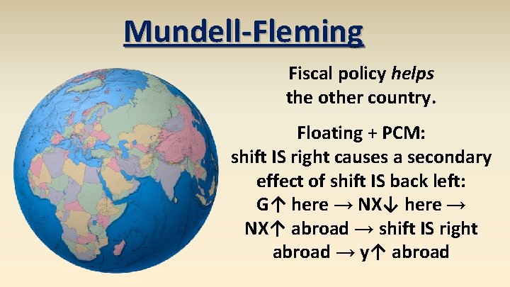
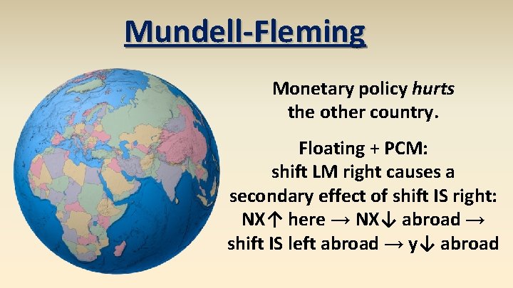
Mundell-Fleming If two countries trade a lot, one country’s policies can effect the other country. With secondary IS curve movements, there is an opposite effect on the other country.

Mundell-Fleming Fiscal policy helps the other country. Floating + PCM: shift IS right causes a secondary effect of shift IS back left: G↑ here → NX↓ here → NX↑ abroad → shift IS right abroad → y↑ abroad

Mundell-Fleming Monetary policy hurts the other country. Floating + PCM: shift LM right causes a secondary effect of shift IS right: NX↑ here → NX↓ abroad → shift IS left abroad → y↓ abroad

Mundell-Fleming This is why the U. S. government strongly encourages other countries to use a fiscal stimulus and strongly discourages other countries from using a monetary stimulus.