Unit 26 Model Assumptions Case Analysis II More

Unit 26: Model Assumptions & Case Analysis II: More complex designs

What is New since Case Analysis I in First Semester • This semester we have focused on how to handle analyses when observations are not completely independent • Four types of designs: 1. Pre-test/post-test designs analyzed with ANCOVA 2. Traditional repeated measures designs with categorical within subject factors. Analyzed with either LM on transformed differences and averages or LMER 3. More advanced repeated measures designs with quantitative within subject factors analyzed in LMER 4. Other designs with dependent data where observations are nested within groups (e. g. , students within classrooms, siblings 2 within families) analyzed with LMER

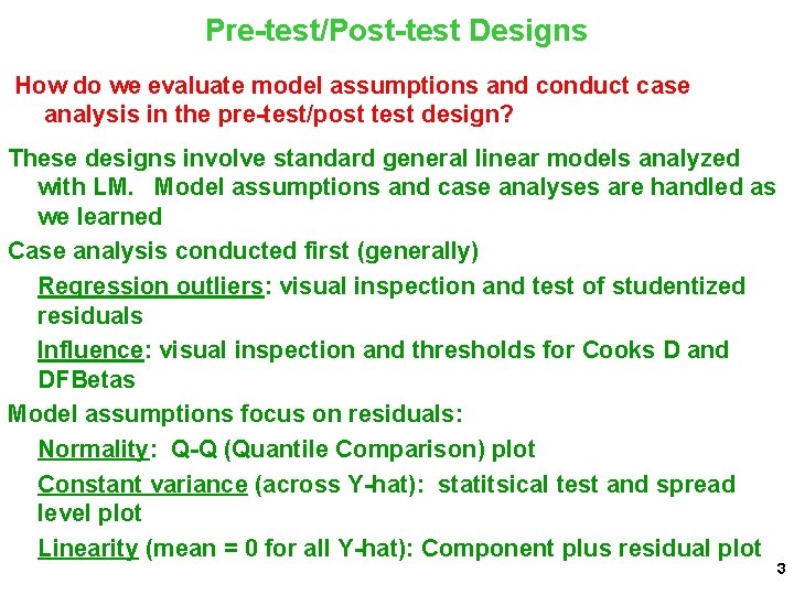
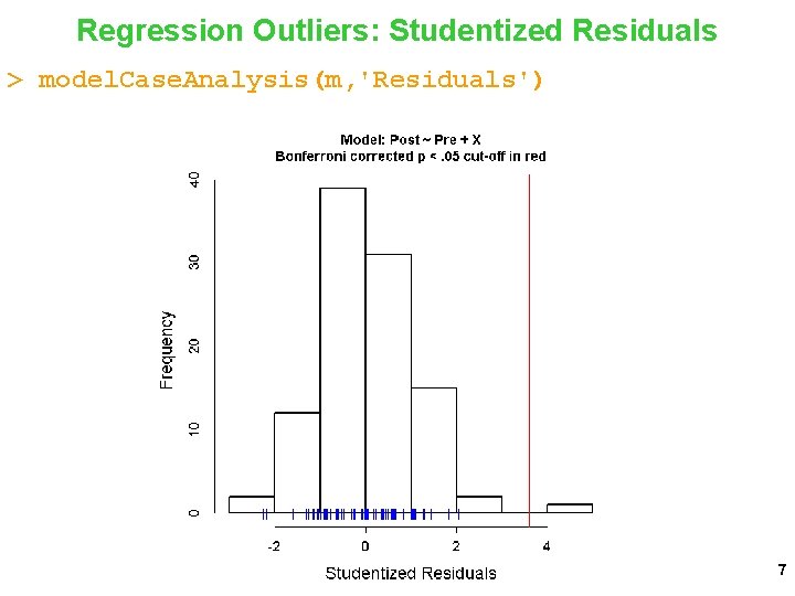
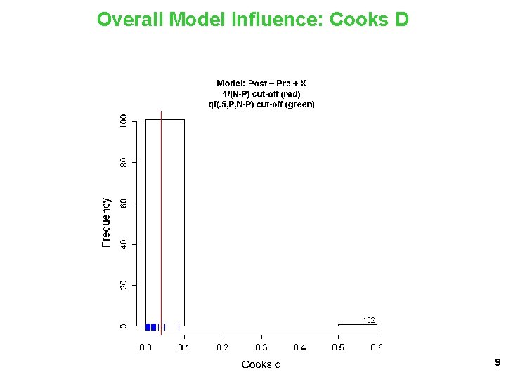
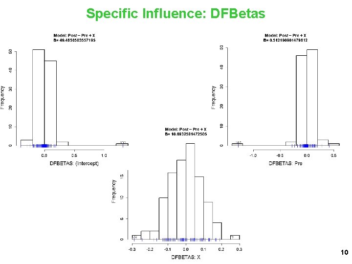
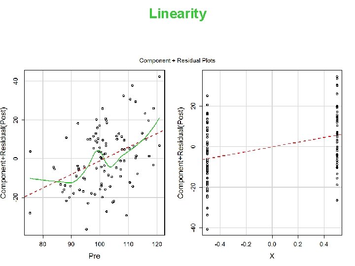
Pre-test/Post-test Designs How do we evaluate model assumptions and conduct case analysis in the pre-test/post test design? These designs involve standard general linear models analyzed with LM. Model assumptions and case analyses are handled as we learned Case analysis conducted first (generally) Regression outliers: visual inspection and test of studentized residuals Influence: visual inspection and thresholds for Cooks D and DFBetas Model assumptions focus on residuals: Normality: Q-Q (Quantile Comparison) plot Constant variance (across Y-hat): statitsical test and spread level plot Linearity (mean = 0 for all Y-hat): Component plus residual plot 3

Pre-test/Post-test design Evaluate a course designed to improve math achievement Measure math achievement at pre-test (before course) Randomly assign to course vs. control group Measure math achievement at post-test How do you analyze, why and what is the critical support for the new course? 4

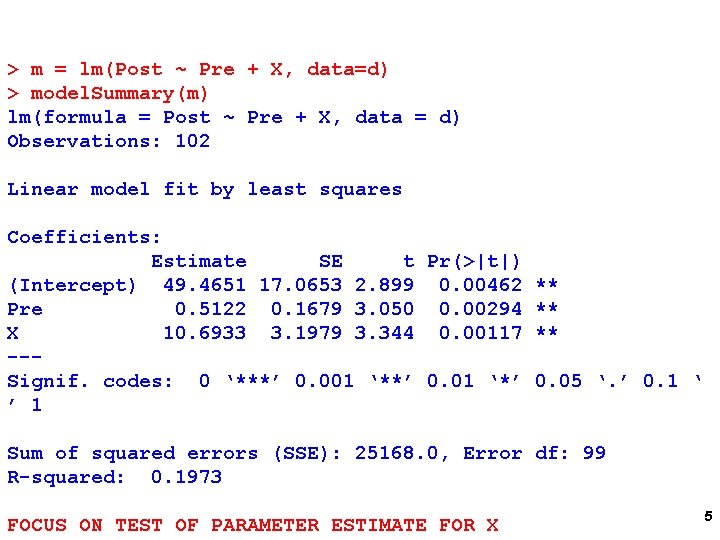
> m = lm(Post ~ Pre + X, data=d) > model. Summary(m) lm(formula = Post ~ Pre + X, data = d) Observations: 102 Linear model fit by least squares Coefficients: Estimate SE t Pr(>|t|) (Intercept) 49. 4651 17. 0653 2. 899 0. 00462 ** Pre 0. 5122 0. 1679 3. 050 0. 00294 ** X 10. 6933 3. 1979 3. 344 0. 00117 ** --Signif. codes: 0 ‘***’ 0. 001 ‘**’ 0. 01 ‘*’ 0. 05 ‘. ’ 0. 1 ‘ ’ 1 Sum of squared errors (SSE): 25168. 0, Error df: 99 R-squared: 0. 1973 FOCUS ON TEST OF PARAMETER ESTIMATE FOR X 5

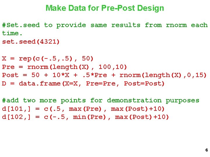
Make Data for Pre-Post Design #Set. seed to provide same results from rnorm each time. set. seed(4321) X = rep(c(-. 5, . 5), 50) Pre = rnorm(length(X), 100, 10) Post = 50 + 10*X +. 5*Pre + rnorm(length(X), 0, 15) D = data. frame(X=X, Pre=Pre, Post=Post) #add two more points for demonstration purposes d[101, ] = c(. 5, max(Pre), max(Post)+10) d[102, ] = c(-. 5, min(Pre), max(Post)+10) 6

Regression Outliers: Studentized Residuals > model. Case. Analysis(m, 'Residuals') 7

Regression Outliers: Studentized Residuals > model. Case. Analysis(m, 'Residuals') 8

Overall Model Influence: Cooks D 9

Specific Influence: DFBetas 10

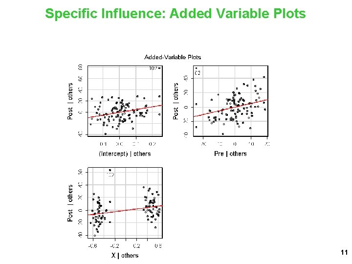
Specific Influence: Added Variable Plots 11

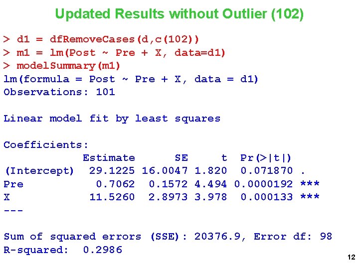
Updated Results without Outlier (102) > d 1 = df. Remove. Cases(d, c(102)) > m 1 = lm(Post ~ Pre + X, data=d 1) > model. Summary(m 1) lm(formula = Post ~ Pre + X, data = d 1) Observations: 101 Linear model fit by least squares Coefficients: Estimate SE t Pr(>|t|) (Intercept) 29. 1225 16. 0047 1. 820 0. 071870. Pre 0. 7062 0. 1572 4. 494 0. 0000192 *** X 11. 5260 2. 8973 3. 978 0. 000133 *** --Sum of squared errors (SSE): 20376. 9, Error df: 98 R-squared: 0. 2986 12

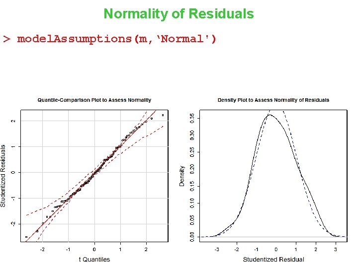
Normality of Residuals > model. Assumptions(m, ‘Normal') 13

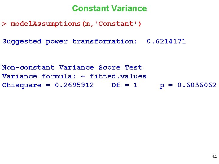
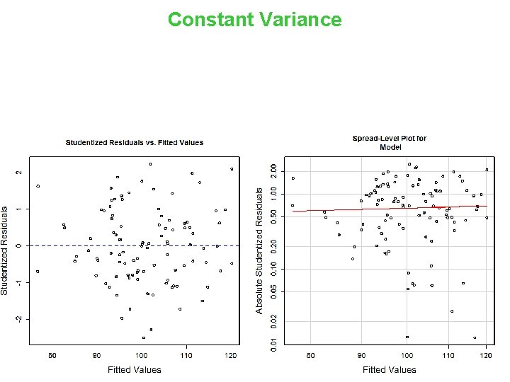
Constant Variance > model. Assumptions(m, 'Constant') Suggested power transformation: Non-constant Variance Score Test Variance formula: ~ fitted. values Chisquare = 0. 2695912 Df = 1 0. 6214171 p = 0. 6036062 14

Constant Variance 15

Linearity 16

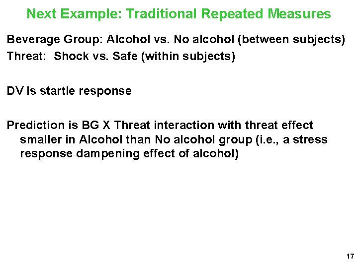
Next Example: Traditional Repeated Measures Beverage Group: Alcohol vs. No alcohol (between subjects) Threat: Shock vs. Safe (within subjects) DV is startle response Prediction is BG X Threat interaction with threat effect smaller in Alcohol than No alcohol group (i. e. , a stress response dampening effect of alcohol) 17

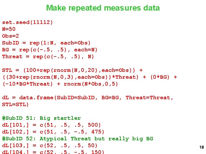
Make repeated measures data set. seed(11112) N=50 Obs=2 Sub. ID = rep(1: N, each=Obs) BG = rep(c(-. 5, . 5), each=N) Threat = rep(c(-. 5, . 5), N) STL = (100+rep(rnorm(N, 0, 20), each=Obs)) + ((30+rep(rnorm(N, 0, 3), each=Obs))*Threat) + (0*BG) + (-10*BG*Threat) + rnorm(N*Obs, 0, 5) d. L = data. frame(Sub. ID=Sub. ID, BG=BG, Threat=Threat, STL=STL) #Sub. ID 51: d. L[101, ] = d. L[102, ] = #Sub. ID 52: d. L[103, ] = Big startler c(51, . 5, 500) c(51, . 5, -. 5, 475) Atypical Threat but really big BG c(52, . 5, 50) 18

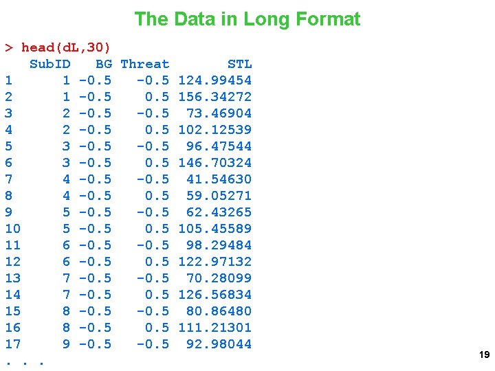
The Data in Long Format > head(d. L, 30) Sub. ID BG Threat STL 1 1 -0. 5 124. 99454 2 1 -0. 5 156. 34272 3 2 -0. 5 73. 46904 4 2 -0. 5 102. 12539 5 3 -0. 5 96. 47544 6 3 -0. 5 146. 70324 7 4 -0. 5 41. 54630 8 4 -0. 5 59. 05271 9 5 -0. 5 62. 43265 10 5 -0. 5 105. 45589 11 6 -0. 5 98. 29484 12 6 -0. 5 122. 97132 13 7 -0. 5 70. 28099 14 7 -0. 5 126. 56834 15 8 -0. 5 80. 86480 16 8 -0. 5 111. 21301 17 9 -0. 5 92. 98044. . . 19

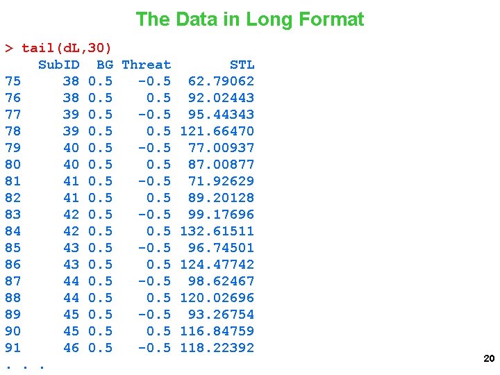
The Data in Long Format > tail(d. L, 30) Sub. ID BG Threat STL 75 38 0. 5 -0. 5 62. 79062 76 38 0. 5 92. 02443 77 39 0. 5 -0. 5 95. 44343 78 39 0. 5 121. 66470 79 40 0. 5 -0. 5 77. 00937 80 40 0. 5 87. 00877 81 41 0. 5 -0. 5 71. 92629 82 41 0. 5 89. 20128 83 42 0. 5 -0. 5 99. 17696 84 42 0. 5 132. 61511 85 43 0. 5 -0. 5 96. 74501 86 43 0. 5 124. 47742 87 44 0. 5 -0. 5 98. 62467 88 44 0. 5 120. 02696 89 45 0. 5 -0. 5 93. 26754 90 45 0. 5 116. 84759 91 46 0. 5 -0. 5 118. 22392. . . 20

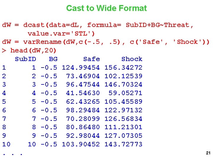
Cast to Wide Format d. W = dcast(data=d. L, formula= Sub. ID+BG~Threat, value. var='STL') d. W = var. Rename(d. W, c(-. 5, . 5), c('Safe', 'Shock')) > head(d. W, 20) Sub. ID BG Safe Shock 1 1 -0. 5 124. 99454 156. 34272 2 2 -0. 5 73. 46904 102. 12539 3 3 -0. 5 96. 47544 146. 70324 4 4 -0. 5 41. 54630 59. 05271 5 5 -0. 5 62. 43265 105. 45589 6 6 -0. 5 98. 29484 122. 97132 7 7 -0. 5 70. 28099 126. 56834 8 8 -0. 5 80. 86480 111. 21301 9 9 -0. 5 92. 98044 127. 07305 10 10 -0. 5 103. 90452 143. 72773 21. . .

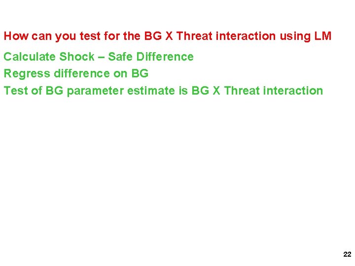
How can you test for the BG X Threat interaction using LM Calculate Shock – Safe Difference Regress difference on BG Test of BG parameter estimate is BG X Threat interaction 22

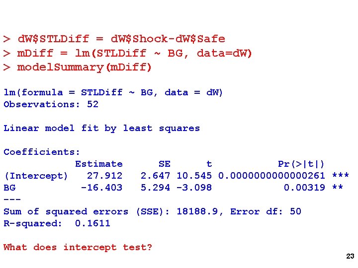
> d. W$STLDiff = d. W$Shock-d. W$Safe > m. Diff = lm(STLDiff ~ BG, data=d. W) > model. Summary(m. Diff) lm(formula = STLDiff ~ BG, data = d. W) Observations: 52 Linear model fit by least squares Coefficients: Estimate SE t Pr(>|t|) (Intercept) 27. 912 2. 647 10. 545 0. 0000000261 *** BG -16. 403 5. 294 -3. 098 0. 00319 ** --Sum of squared errors (SSE): 18188. 9, Error df: 50 R-squared: 0. 1611 What does intercept test? 23

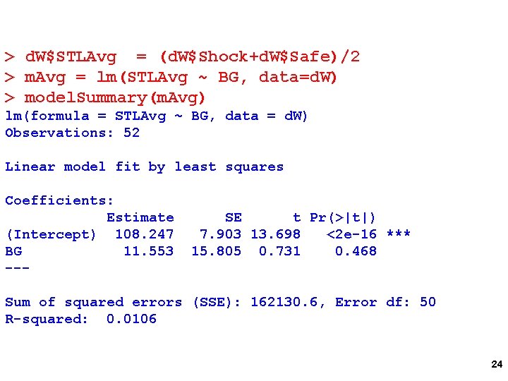
> d. W$STLAvg = (d. W$Shock+d. W$Safe)/2 > m. Avg = lm(STLAvg ~ BG, data=d. W) > model. Summary(m. Avg) lm(formula = STLAvg ~ BG, data = d. W) Observations: 52 Linear model fit by least squares Coefficients: Estimate (Intercept) 108. 247 BG 11. 553 --- SE t Pr(>|t|) 7. 903 13. 698 <2 e-16 *** 15. 805 0. 731 0. 468 Sum of squared errors (SSE): 162130. 6, Error df: 50 R-squared: 0. 0106 24

Your experiment focused on the BG X Threat interaction. You want to report the test of that parameter estimate with confidence. What do you do? Evaluate model assumptions and do case analysis on the m. Diff model. This is just a simple linear regression in LM. You know exactly what to do. 25

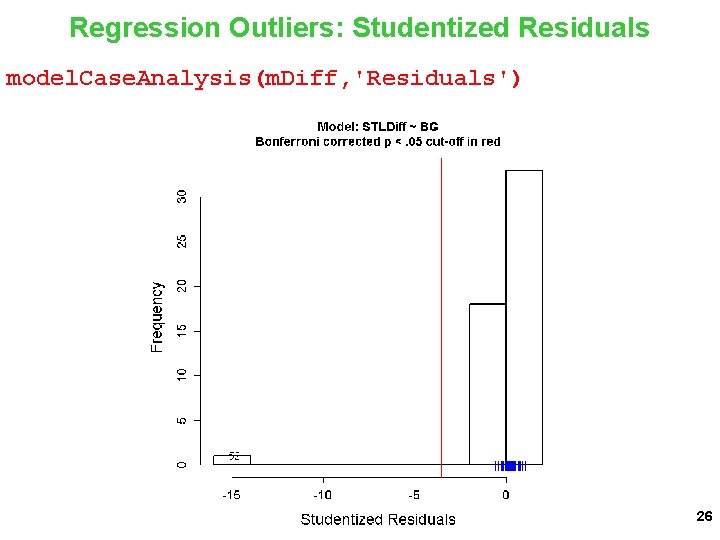
Regression Outliers: Studentized Residuals model. Case. Analysis(m. Diff, 'Residuals') 26

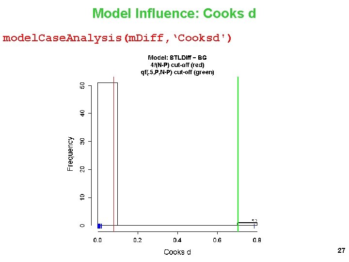
Model Influence: Cooks d model. Case. Analysis(m. Diff, ‘Cooksd') 27

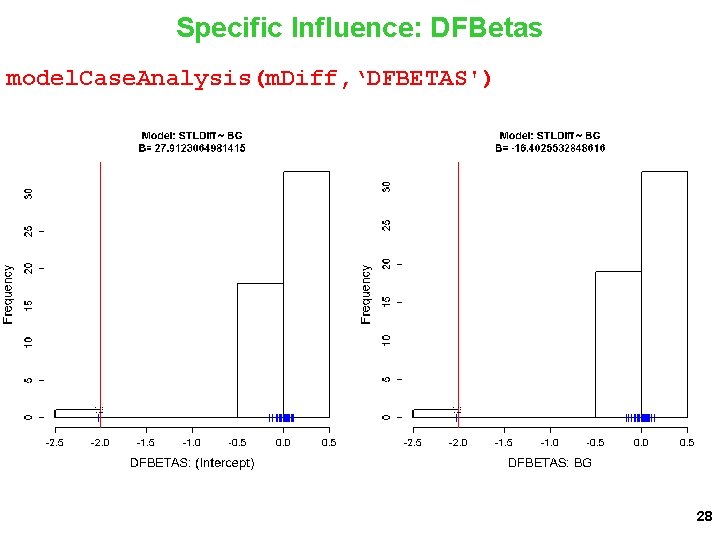
Specific Influence: DFBetas model. Case. Analysis(m. Diff, ‘DFBETAS') 28

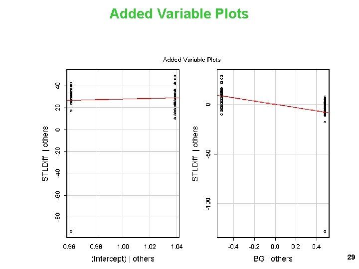
Added Variable Plots 29

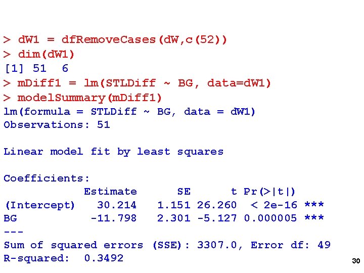
> d. W 1 = df. Remove. Cases(d. W, c(52)) > dim(d. W 1) [1] 51 6 > m. Diff 1 = lm(STLDiff ~ BG, data=d. W 1) > model. Summary(m. Diff 1) lm(formula = STLDiff ~ BG, data = d. W 1) Observations: 51 Linear model fit by least squares Coefficients: Estimate SE t Pr(>|t|) (Intercept) 30. 214 1. 151 26. 260 < 2 e-16 *** BG -11. 798 2. 301 -5. 127 0. 000005 *** --Sum of squared errors (SSE): 3307. 0, Error df: 49 R-squared: 0. 3492 30

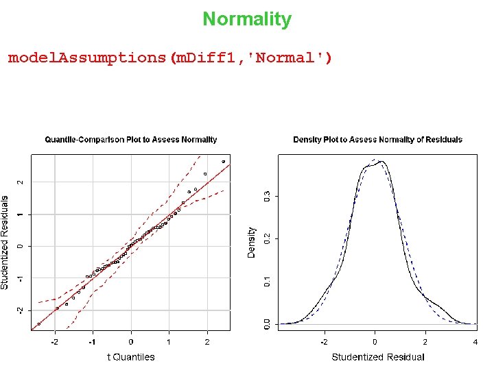
Normality model. Assumptions(m. Diff 1, 'Normal') 31

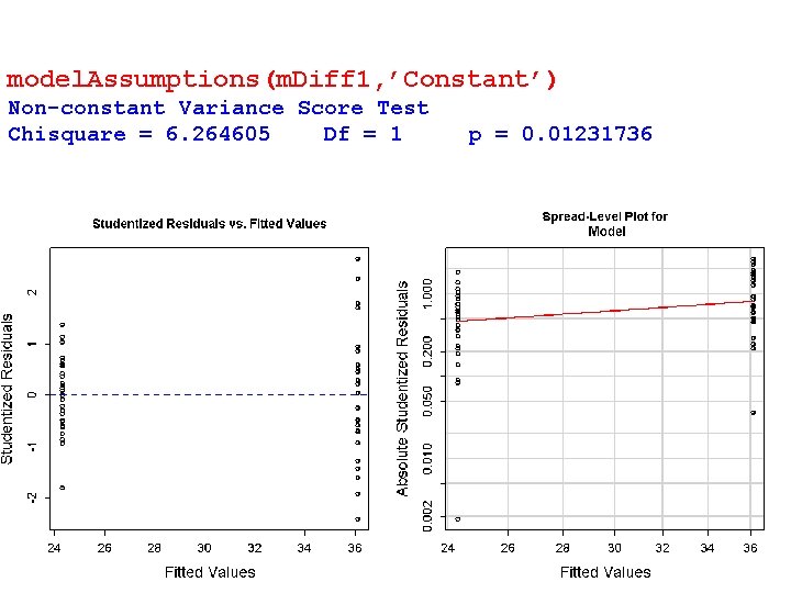
model. Assumptions(m. Diff 1, ’Constant’) Non-constant Variance Score Test Chisquare = 6. 264605 Df = 1 p = 0. 01231736 32

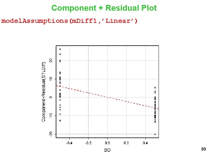
Component + Residual Plot model. Assumptions(m. Diff 1, ’Linear’) 33

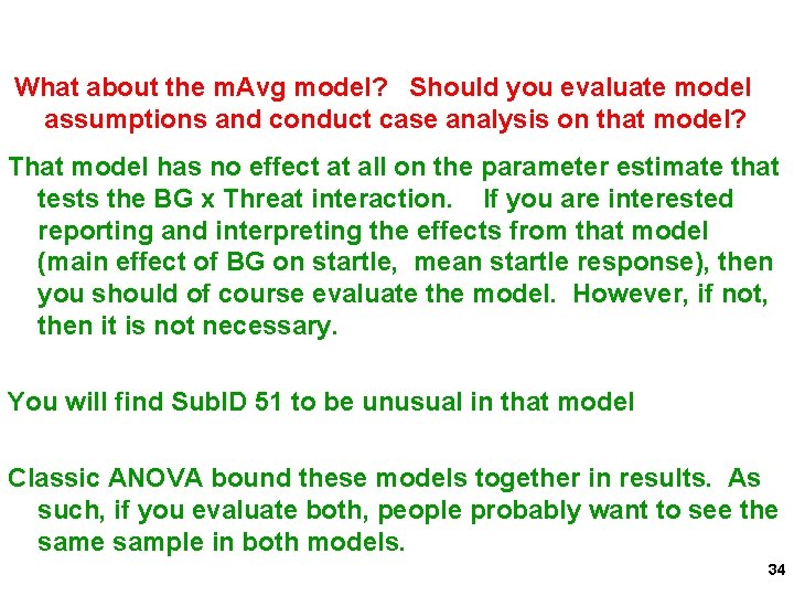
What about the m. Avg model? Should you evaluate model assumptions and conduct case analysis on that model? That model has no effect at all on the parameter estimate that tests the BG x Threat interaction. If you are interested reporting and interpreting the effects from that model (main effect of BG on startle, mean startle response), then you should of course evaluate the model. However, if not, then it is not necessary. You will find Sub. ID 51 to be unusual in that model Classic ANOVA bound these models together in results. As such, if you evaluate both, people probably want to see the sample in both models. 34

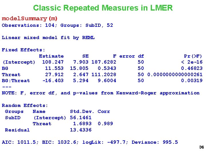
Classic Repeated Measures in LMER m = lmer(STL ~ BG*Threat + (1+Threat|Sub. ID), data=d. L, control= lmer. Control(check. nobs. vs. n. RE="ignore")) 35

Classic Repeated Measures in LMER model. Summary(m) Observations: 104; Groups: Sub. ID, 52 Linear mixed model fit by REML Fixed Effects: Estimate SE F error df Pr(>F) (Intercept) 108. 247 7. 903 187. 6282 50 < 2 e-16 BG 11. 553 15. 805 0. 5343 50 0. 46823 Threat 27. 912 2. 647 111. 2028 50 0. 0000000261 BG: Threat -16. 403 5. 294 9. 6004 50 0. 00319 --NOTE: F, error df, and p-values from Kenward-Roger approximation Random Effects: Groups Name Std. Dev. Corr Sub. ID (Intercept) 56. 1461 Threat 1. 6893 0. 989 Residual 13. 4336 AIC: 1011. 5; BIC: 1032. 6; log. Lik: -497. 7; Deviance: 995. 5 36

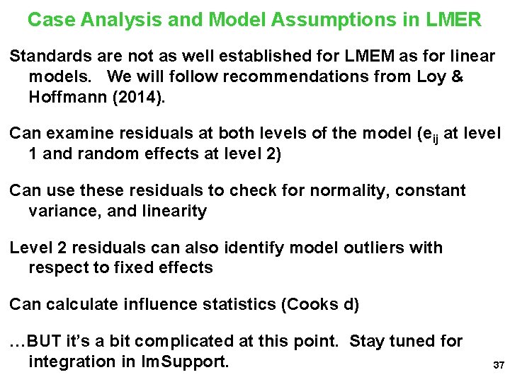
Case Analysis and Model Assumptions in LMER Standards are not as well established for LMEM as for linear models. We will follow recommendations from Loy & Hoffmann (2014). Can examine residuals at both levels of the model (eij at level 1 and random effects at level 2) Can use these residuals to check for normality, constant variance, and linearity Level 2 residuals can also identify model outliers with respect to fixed effects Can calculate influence statistics (Cooks d) …BUT it’s a bit complicated at this point. Stay tuned for integration in lm. Support. 37

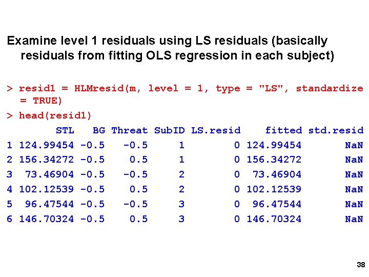
Examine level 1 residuals using LS residuals (basically residuals from fitting OLS regression in each subject) > resid 1 = HLMresid(m, level = 1, type = TRUE) > head(resid 1) STL BG Threat Sub. ID LS. resid 1 124. 99454 -0. 5 1 0 2 156. 34272 -0. 5 1 0 3 73. 46904 -0. 5 2 0 4 102. 12539 -0. 5 2 0 5 96. 47544 -0. 5 3 0 6 146. 70324 -0. 5 3 0 = "LS", standardize fitted std. resid 124. 99454 Na. N 156. 34272 Na. N 73. 46904 Na. N 102. 12539 Na. N 96. 47544 Na. N 146. 70324 Na. N 38

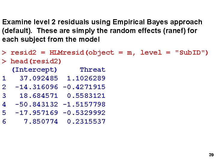
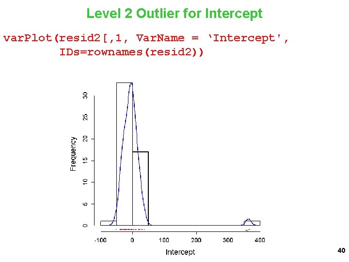
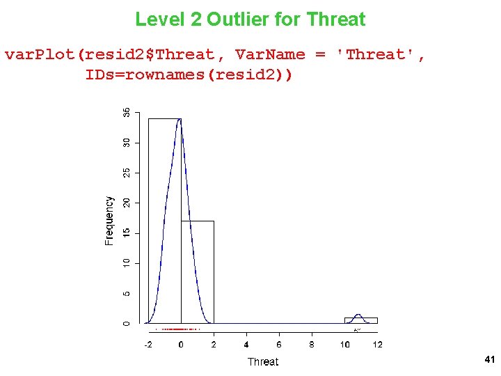
Examine level 2 residuals using Empirical Bayes approach (default). These are simply the random effects (ranef) for each subject from the model > resid 2 = HLMresid(object = m, level = "Sub. ID") > head(resid 2) (Intercept) Threat 1 37. 092485 1. 1026289 2 -14. 316096 -0. 4271915 3 18. 684571 0. 5583121 4 -50. 843132 -1. 5157798 5 -17. 957169 -0. 5329992 6 7. 850774 0. 2315537 39

Level 2 Outlier for Intercept var. Plot(resid 2[, 1, Var. Name = ‘Intercept', IDs=rownames(resid 2)) 40

Level 2 Outlier for Threat var. Plot(resid 2$Threat, Var. Name = 'Threat', IDs=rownames(resid 2)) 41

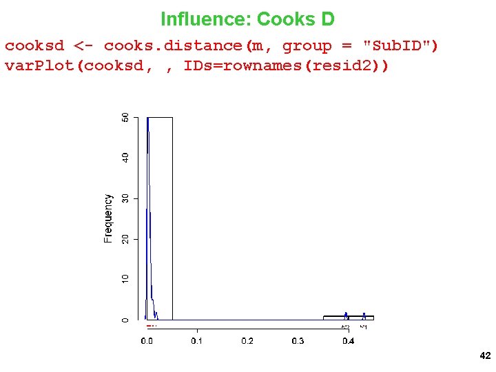
Influence: Cooks D cooksd <- cooks. distance(m, group = "Sub. ID") var. Plot(cooksd, , IDs=rownames(resid 2)) 42

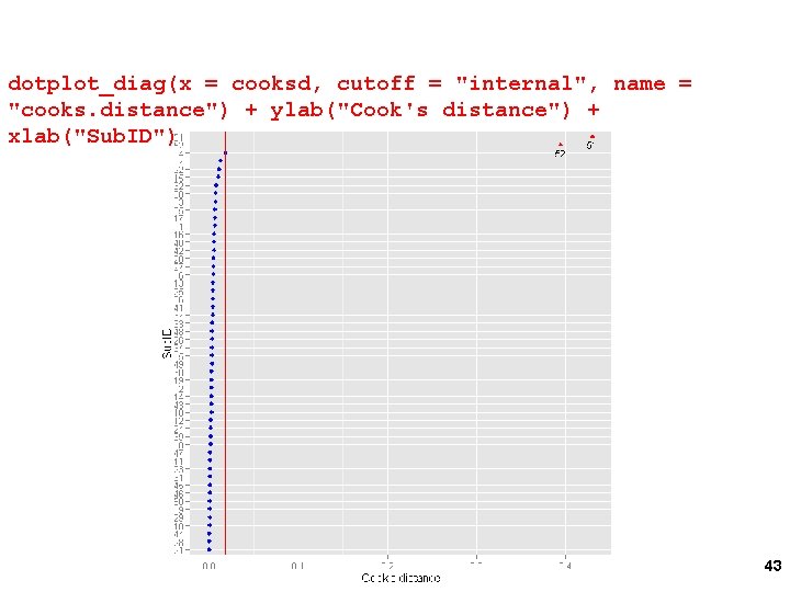
dotplot_diag(x = cooksd, cutoff = "internal", name = "cooks. distance") + ylab("Cook's distance") + xlab("Sub. ID") 43

Quantifying Parameter Estimate Change beta_51 = as. numeric(attr(cooksd, "beta_cdd")[[51]]) names(beta_51) <- names(fixef(m)) beta_52 = as. numeric(attr(cooksd, "beta_cdd")[[52]]) names(beta_52) <- names(fixef(m)) fixef(m) (Intercept) 108. 24711 BG 11. 55264 Threat 27. 91231 BG: Threat -16. 40255 beta_51 #This subject increases intercept and BG (Intercept) BG Threat BG: Threat 7. 1822417 14. 3644833 0. 1017110 0. 2034219 beta_52 #This subject decreases threat and increases (more negative) interaction (Intercept) BG Threat BG: Threat 44 -0. 2696814 -0. 5393629 -2. 3021352 -4. 6042704

Normality for Random Intercept ggplot_qqnorm(x = resid 2[, 1], line = "rlm") 45

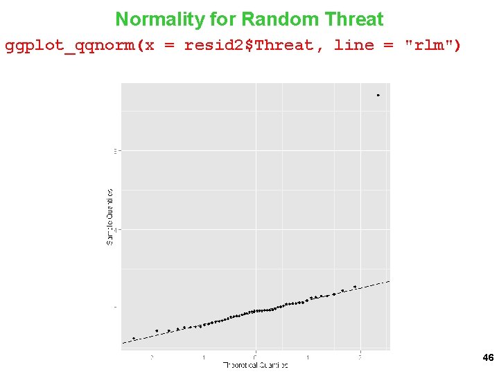
Normality for Random Threat ggplot_qqnorm(x = resid 2$Threat, line = "rlm") 46

TRUE LMEM Threat: Safe vs. Shock Trial 1 -20 DV is startle Focus on Trial X Threat interaction 47

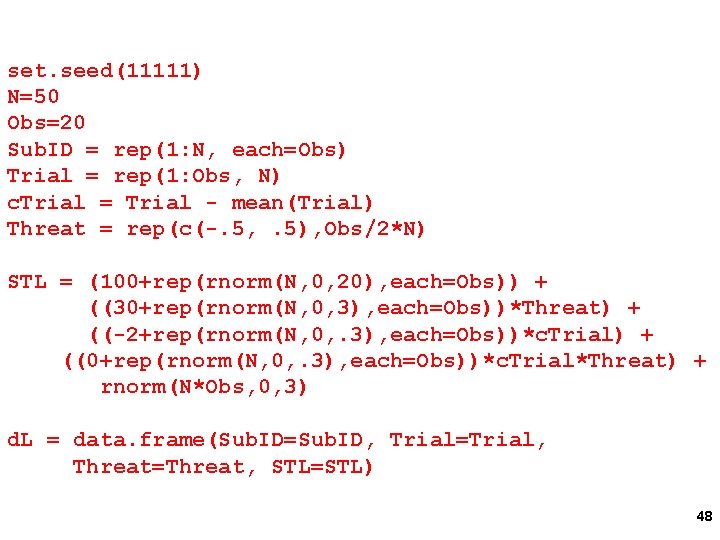
set. seed(11111) N=50 Obs=20 Sub. ID = rep(1: N, each=Obs) Trial = rep(1: Obs, N) c. Trial = Trial - mean(Trial) Threat = rep(c(-. 5, . 5), Obs/2*N) STL = (100+rep(rnorm(N, 0, 20), each=Obs)) + ((30+rep(rnorm(N, 0, 3), each=Obs))*Threat) + ((-2+rep(rnorm(N, 0, . 3), each=Obs))*c. Trial) + ((0+rep(rnorm(N, 0, . 3), each=Obs))*c. Trial*Threat) + rnorm(N*Obs, 0, 3) d. L = data. frame(Sub. ID=Sub. ID, Trial=Trial, Threat=Threat, STL=STL) 48

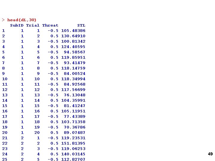
> head(d. L, 30) Sub. ID Trial Threat STL 1 1 1 -0. 5 105. 48386 2 1 2 0. 5 130. 64910 3 1 3 -0. 5 100. 81342 4 1 4 0. 5 124. 40595 5 1 5 -0. 5 94. 58567 6 1 6 0. 5 119. 85951 7 -0. 5 93. 41479 8 1 8 0. 5 118. 14759 9 1 9 -0. 5 84. 00524 10 1 10 0. 5 118. 34994 11 1 11 -0. 5 84. 92568 12 1 12 0. 5 117. 56699 13 1 13 -0. 5 76. 13048 14 1 14 0. 5 104. 35991 15 -0. 5 81. 41247 16 1 16 0. 5 105. 11951 17 -0. 5 77. 43389 18 1 18 0. 5 103. 71358 19 1 19 -0. 5 70. 36786 20 1 20 0. 5 89. 07487 21 2 1 -0. 5 119. 23531 22 2 2 0. 5 151. 81395 23 2 3 -0. 5 119. 06253 24 2 4 0. 5 140. 03145 25 2 5 -0. 5 112. 82707 49

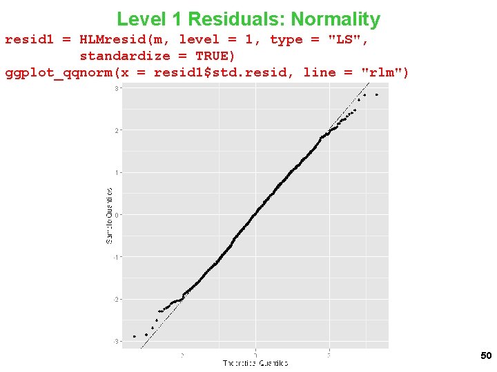
Level 1 Residuals: Normality resid 1 = HLMresid(m, level = 1, type = "LS", standardize = TRUE) ggplot_qqnorm(x = resid 1$std. resid, line = "rlm") 50

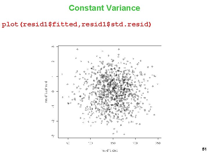
Constant Variance plot(resid 1$fitted, resid 1$std. resid) 51

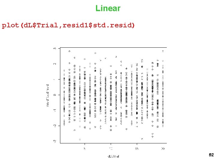
Linear plot(d. L$Trial, resid 1$std. resid) 52

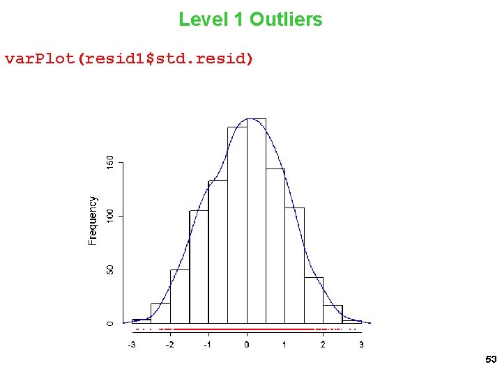
Level 1 Outliers var. Plot(resid 1$std. resid) 53

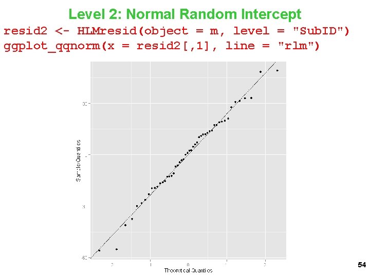
Level 2: Normal Random Intercept resid 2 <- HLMresid(object = m, level = "Sub. ID") ggplot_qqnorm(x = resid 2[, 1], line = "rlm") 54

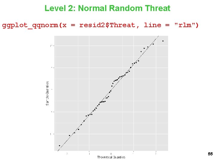
Level 2: Normal Random Threat ggplot_qqnorm(x = resid 2$Threat, line = "rlm") 55

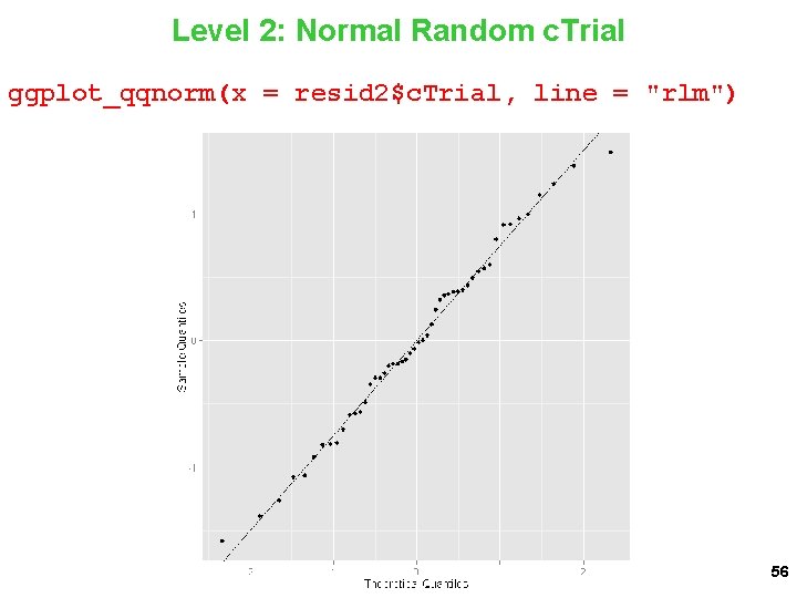
Level 2: Normal Random c. Trial ggplot_qqnorm(x = resid 2$c. Trial, line = "rlm") 56

Level 2: Normal Random Threat: c. Trial ggplot_qqnorm(x = resid 2[, 4], line = "rlm") 57

Level 2 Outliers: c. Trial: Threat ggplot_qqnorm(x = resid 2[, 4], line = "rlm") 58

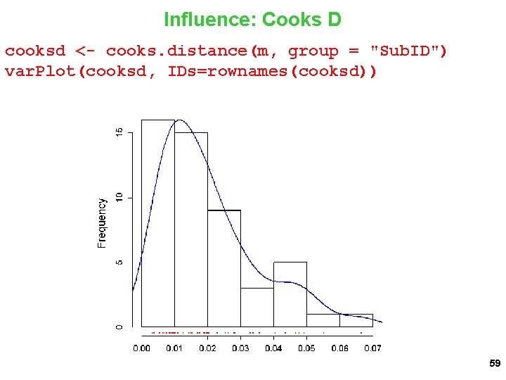
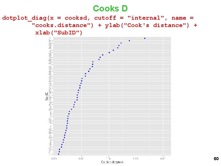
Influence: Cooks D cooksd <- cooks. distance(m, group = "Sub. ID") var. Plot(cooksd, IDs=rownames(cooksd)) 59

Cooks D dotplot_diag(x = cooksd, cutoff = "internal", name = "cooks. distance") + ylab("Cook's distance") + xlab("Sub. ID") 60