Unit 22 Repeated Measures Designs Review Design Considerations

Unit 22: Repeated Measures Designs: Review, Design Considerations, and an Alternative Approach

Unit Goals Further review of standard repeated measures analyses via lm and lmer (conceptual and practical) Consider design issues in repeated measures Introduce alternative (not statistically equivalent) approach to analysis of repeated measures Compare and contrast alternative approach with lm/lmer. Which should you use when and why? 2

Repeated Measures Designs: A Detailed Review What are the cardinal feature(s) of a repeated measures (within-subject) design? You have more than one observation per unit of analysis. Most typically, you have more than one observation per participant (as participant is our typical unit of analysis). You have the same units (e. g. , participants) in all conditions associated with a within-subject independent variable in your experiment. Give two examples: Fully within subject and mixed designs? What are the advantages of a repeated measures design? In most instances*, you will have more power than the comparable between subjects design with the same N It is more efficient use of N when subjects are difficult to find 3 Allows you to examine change over time within participants 3

Repeated Measures Designs: A Detailed Review What problems or barriers exist with repeated measures designs? Can’t manipulate IV (e. g. , Sex, Alcohol Dependence) Contamination of IV conditions Order effects (e. g. , practice, fatigue) Cannot counterbalance conditions (e. g. , cant take away treatment once given) Can counterbalance but Order effects are large- Why is this a problem? What are the consequences of each of these problems? Cant manipulate- Cant do it! Contamination- decrease internal validity, decrease statistical validity (power) Order effects- decrease internal validity (not counterbalanced) or decrease statistical power (counterbalanced but large, unmodeled 4 order effects) 4

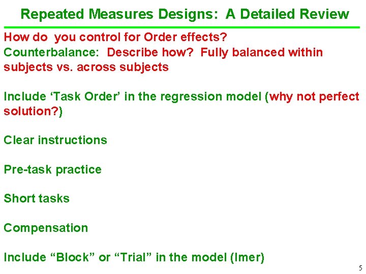
Repeated Measures Designs: A Detailed Review How do you control for Order effects? Counterbalance: Describe how? Fully balanced within subjects vs. across subjects Include ‘Task Order’ in the regression model (why not perfect solution? ) Clear instructions Pre-task practice Short tasks Compensation Include “Block” or “Trial” in the model (lmer) 5 5

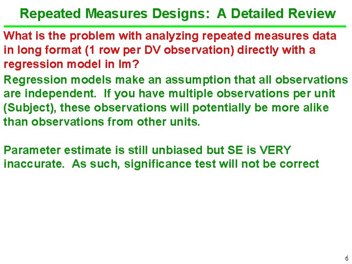
Repeated Measures Designs: A Detailed Review What is the problem with analyzing repeated measures data in long format (1 row per DV observation) directly with a regression model in lm? Regression models make an assumption that all observations are independent. If you have multiple observations per unit (Subject), these observations will potentially be more alike than observations from other units. Parameter estimate is still unbiased but SE is VERY inaccurate. As such, significance test will not be correct 6

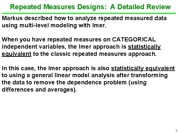
Repeated Measures Designs: A Detailed Review Markus described how to analyze repeated measured data using multi-level modeling with lmer. When you have repeated measures on CATEGORICAL independent variables, the lmer approach is statistically equivalent to the classic repeated measures approach. In this case, the lmer approach is also statistically equivalent to using a general linear model analysis after transforming the data to remove the dependence problem (using differences and averages). 7

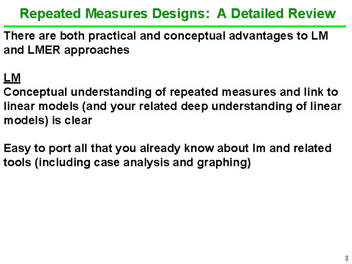
Repeated Measures Designs: A Detailed Review There are both practical and conceptual advantages to LM and LMER approaches LM Conceptual understanding of repeated measures and link to linear models (and your related deep understanding of linear models) is clear Easy to port all that you already know about lm and related tools (including case analysis and graphing) 8 8

Repeated Measures Designs: A Detailed Review LMER Much easier (less code) to execute in R. Only one unified output (will be made even easier in future version of lm. Support) Data structure makes sense and matches traditional between subjects case. Within and between subject IV contrasts all handled in the same way Conceptual link to multi-level modeling is very attractive. Repeated measures is a simple example of a multi-level model but there are many other designs that multi-level models are well suited. These more complex designs can be applied to repeated measures designs but also to other designs (e. g. , students in classes; multiple observations 9 over time with interest in change of time) 9

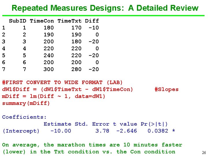
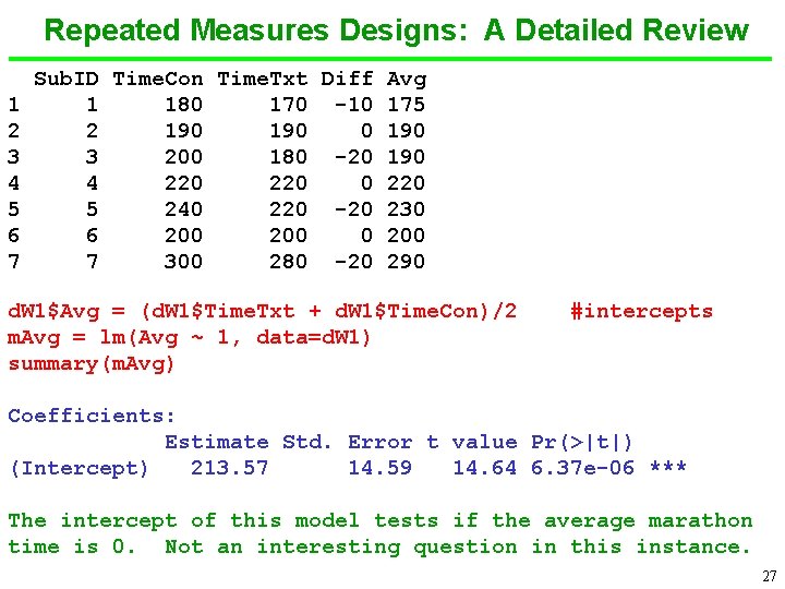
Repeated Measures Designs: A Detailed Review Describe how to fix the independence problem in a design with one within subject variable with two levels? Describe this such that you can accomplish the analyses in lm 1. Calculate the difference between the two measurements for each subject (these are the slopes from the level 1 lmer approach). 2. Calculate the average of the two measurements for each subject (these are the intercepts from the level 1 lmer approach) 3. Estimate two regression models. One of these models will have the differences/slopes as the DV. The second will have the averages/intercepts as the DV. 4. All relevant effects (and some “irrelevant” effects) will be provided by the tests of the regression coefficients across 10 these two models 10

Repeated Measures Designs: A Detailed Review How does this fix the independence problem? Each regression model only has 1 observation per unit (participant) so all observations are now independent The use of difference and average methods to remove the dependence was intentional because each has a meaningful interpretation. The difference (slope) method indexes change in original dependent measure across levels of the within subject variable The average (intercept) method indexes the overall level of original dependent measure 11 11

Repeated Measures Designs: A Detailed Review Blood doping is the practice of boosting the number of red blood cells in the bloodstream in order to enhance athletic performance. Because such blood cells carry oxygen from the lungs to the muscles, a higher concentration in the blood may improve an athlete’s aerobic capacity (VO 2 max) and endurance. Does blood doping work for marathon runners? Sketch the important design features of the experiment briefly At a minimum, consider issues related to the treatment/control groups (between/within, blinding, length/dose of txt, multiple doses), characteristics of the population to study, selection of DV, N 12 12

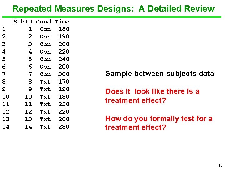
Repeated Measures Designs: A Detailed Review 1 2 3 4 5 6 7 8 9 10 11 12 13 14 Sub. ID Cond Time 1 Con 180 2 Con 190 3 Con 200 4 Con 220 5 Con 240 6 Con 200 7 Con 300 8 Txt 170 9 Txt 190 10 Txt 180 11 Txt 220 12 Txt 220 13 Txt 200 14 Txt 280 Sample between subjects data Does it look like there is a treatment effect? How do you formally test for a treatment effect? 13 13

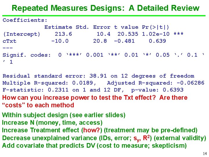
Repeated Measures Designs: A Detailed Review Coefficients: Estimate Std. Error t value Pr(>|t|) (Intercept) 213. 6 10. 4 20. 535 1. 02 e-10 *** c. Txt -10. 0 20. 8 -0. 481 0. 639 --Signif. codes: 0 ‘***’ 0. 001 ‘**’ 0. 01 ‘*’ 0. 05 ‘. ’ 0. 1 ‘ ’ 1 Residual standard error: 38. 91 on 12 degrees of freedom Multiple R-squared: 0. 0189, Adjusted R-squared: -0. 06286 F-statistic: 0. 2311 on 1 and 12 DF, p-value: 0. 6393 How can you increase power to test the Txt effect? Are there “costs” to each method Within subject design (see earlier slides) Increase N (money, time, access) Increase Treatment effect (how? ) (treatment may be pre-defined) Decrease unexplained variance (IDs, error; sy, R 2) (external validity) Add covariate that predicts DV (cost to measure; skepticism) 14 14

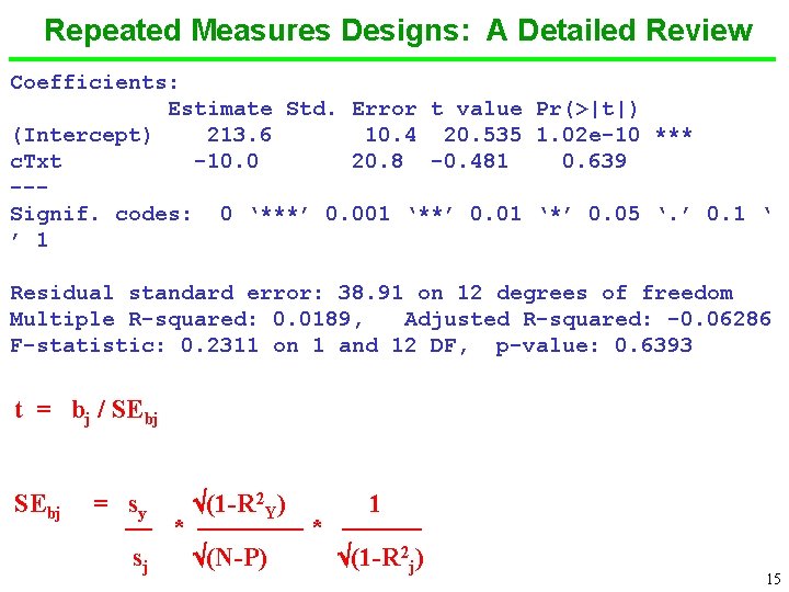
Repeated Measures Designs: A Detailed Review Coefficients: Estimate Std. Error t value Pr(>|t|) (Intercept) 213. 6 10. 4 20. 535 1. 02 e-10 *** c. Txt -10. 0 20. 8 -0. 481 0. 639 --Signif. codes: 0 ‘***’ 0. 001 ‘**’ 0. 01 ‘*’ 0. 05 ‘. ’ 0. 1 ‘ ’ 1 Residual standard error: 38. 91 on 12 degrees of freedom Multiple R-squared: 0. 0189, Adjusted R-squared: -0. 06286 F-statistic: 0. 2311 on 1 and 12 DF, p-value: 0. 6393 t = bj / SEbj = sy (1 -R 2 Y) 1 — * ——— sj (N-P) (1 -R 2 j) 15

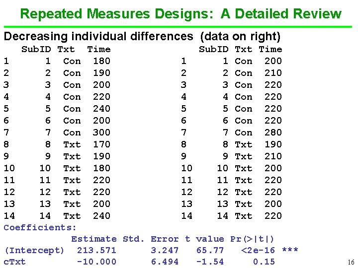
Repeated Measures Designs: A Detailed Review Decreasing individual differences (data on right) 1 2 3 4 5 6 7 8 9 10 11 12 13 14 Sub. ID Txt Time 1 Con 180 2 Con 190 3 Con 200 4 Con 220 5 Con 240 6 Con 200 7 Con 300 8 Txt 170 9 Txt 190 10 Txt 180 11 Txt 220 12 Txt 220 13 Txt 200 14 Txt 240 1 2 3 4 5 6 7 8 9 10 11 12 13 14 Sub. ID 1 2 3 4 5 6 7 8 9 10 11 12 13 14 Txt Time Con 200 Con 210 Con 220 Con 280 Txt 190 Txt 210 Txt 200 Txt 220 Coefficients: Estimate Std. Error t value Pr(>|t|) (Intercept) 213. 571 3. 247 65. 77 <2 e-16 *** c. Txt -10. 000 6. 494 -1. 54 0. 15 16

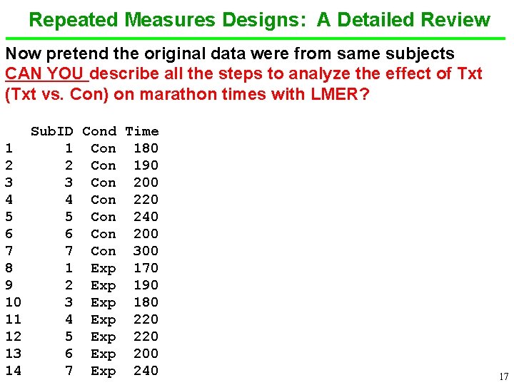
Repeated Measures Designs: A Detailed Review Now pretend the original data were from same subjects CAN YOU describe all the steps to analyze the effect of Txt (Txt vs. Con) on marathon times with LMER? 1 2 3 4 5 6 7 8 9 10 11 12 13 14 Sub. ID Cond Time 1 Con 180 2 Con 190 3 Con 200 4 Con 220 5 Con 240 6 Con 200 7 Con 300 1 Exp 170 2 Exp 190 3 Exp 180 4 Exp 220 5 Exp 220 6 Exp 200 7 Exp 240 17

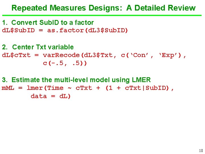
Repeated Measures Designs: A Detailed Review 1. Convert Sub. ID to a factor d. L$Sub. ID = as. factor(d. L 3$Sub. ID) 2. Center Txt variable d. L$c. Txt = var. Recode(d. L 3$Txt, c(‘Con’, ‘Exp’), c(-. 5, . 5)) 3. Estimate the multi-level model using LMER m. ML = lmer(Time ~ c. Txt + (1 + c. Txt|Sub. ID), data = d. L) 18

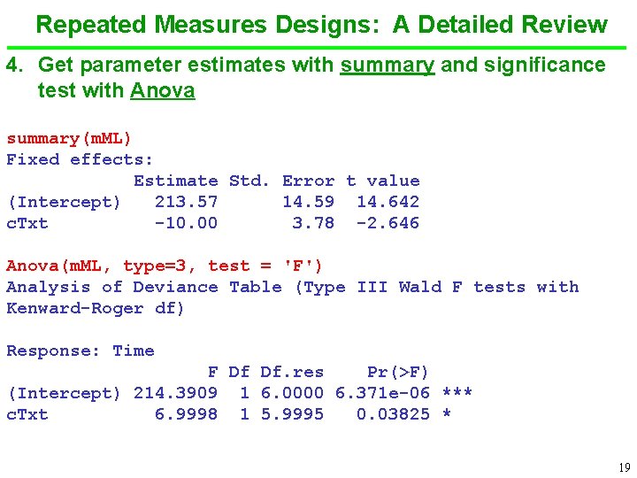
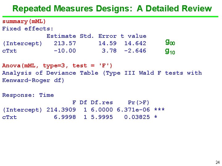
Repeated Measures Designs: A Detailed Review 4. Get parameter estimates with summary and significance test with Anova summary(m. ML) Fixed effects: Estimate Std. Error t value (Intercept) 213. 57 14. 59 14. 642 c. Txt -10. 00 3. 78 -2. 646 Anova(m. ML, type=3, test = 'F') Analysis of Deviance Table (Type III Wald F tests with Kenward-Roger df) Response: Time F Df Df. res Pr(>F) (Intercept) 214. 3909 1 6. 0000 6. 371 e-06 *** c. Txt 6. 9998 1 5. 9995 0. 03825 * 19

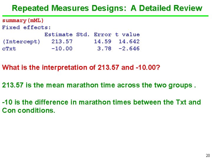
Repeated Measures Designs: A Detailed Review summary(m. ML) Fixed effects: Estimate Std. Error t value (Intercept) 213. 57 14. 59 14. 642 c. Txt -10. 00 3. 78 -2. 646 What is the interpretation of 213. 57 and -10. 00? 213. 57 is the mean marathon time across the two groups. -10 is the difference in marathon times between the Txt and Con conditions. 20

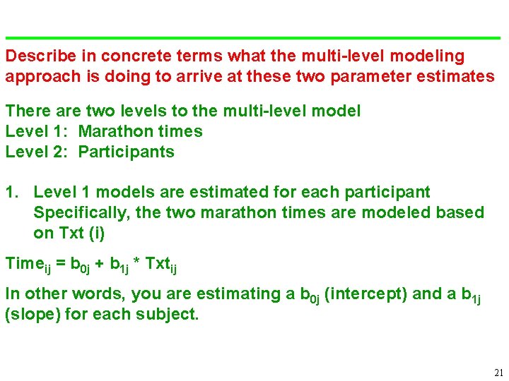
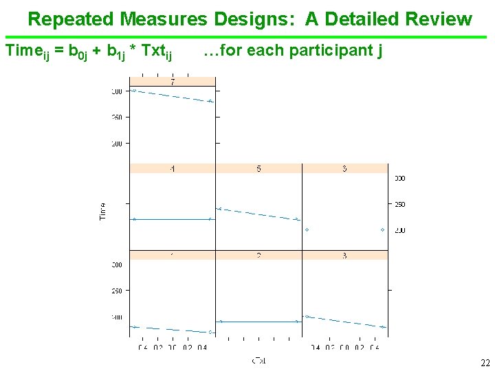
Describe in concrete terms what the multi-level modeling approach is doing to arrive at these two parameter estimates There are two levels to the multi-level model Level 1: Marathon times Level 2: Participants 1. Level 1 models are estimated for each participant Specifically, the two marathon times are modeled based on Txt (i) Timeij = b 0 j + b 1 j * Txtij In other words, you are estimating a b 0 j (intercept) and a b 1 j (slope) for each subject. 21

Repeated Measures Designs: A Detailed Review Timeij = b 0 j + b 1 j * Txtij …for each participant j 22 22

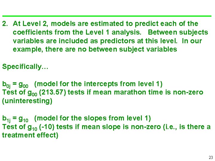
2. At Level 2, models are estimated to predict each of the coefficients from the Level 1 analysis. Between subjects variables are included as predictors at this level. In our example, there are no between subject variables Specifically… b 0 j = g 00 (model for the intercepts from level 1) Test of g 00 (213. 57) tests if mean marathon time is non-zero (uninteresting) b 1 j = g 10 (model for the slopes from level 1) Test of g 10 (-10) tests if mean slope is non-zero (i. e. , is there a treatment effect) 23

Repeated Measures Designs: A Detailed Review summary(m. ML) Fixed effects: Estimate Std. Error t value (Intercept) 213. 57 14. 59 14. 642 c. Txt -10. 00 3. 78 -2. 646 g 00 g 10 Anova(m. ML, type=3, test = 'F') Analysis of Deviance Table (Type III Wald F tests with Kenward-Roger df) Response: Time F Df Df. res Pr(>F) (Intercept) 214. 3909 1 6. 0000 6. 371 e-06 *** c. Txt 6. 9998 1 5. 9995 0. 03825 * 24

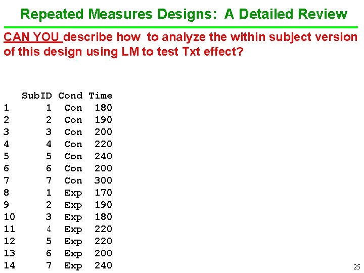
Repeated Measures Designs: A Detailed Review CAN YOU describe how to analyze the within subject version of this design using LM to test Txt effect? 1 2 3 4 5 6 7 8 9 10 11 12 13 14 Sub. ID Cond Time 1 Con 180 2 Con 190 3 Con 200 4 Con 220 5 Con 240 6 Con 200 7 Con 300 1 Exp 170 2 Exp 190 3 Exp 180 4 Exp 220 5 Exp 220 6 Exp 200 7 Exp 240 25

Repeated Measures Designs: A Detailed Review 1 2 3 4 5 6 7 Sub. ID Time. Con Time. Txt Diff 1 180 170 -10 2 190 0 3 200 180 -20 4 220 0 5 240 220 -20 6 200 0 7 300 280 -20 #FIRST CONVERT TO WIDE FORMAT (LAB) d. W 1$Diff = (d. W 1$Time. Txt - d. W 1$Time. Con) m. Diff = lm(Diff ~ 1, data=d. W 1) summary(m. Diff) #Slopes Coefficients: Estimate Std. Error t value Pr(>|t|) (Intercept) -10. 00 3. 78 -2. 646 0. 0382 * On average, the marathon times are 10 minutes faster (lower) in the Txt condition vs. the Con condition 26

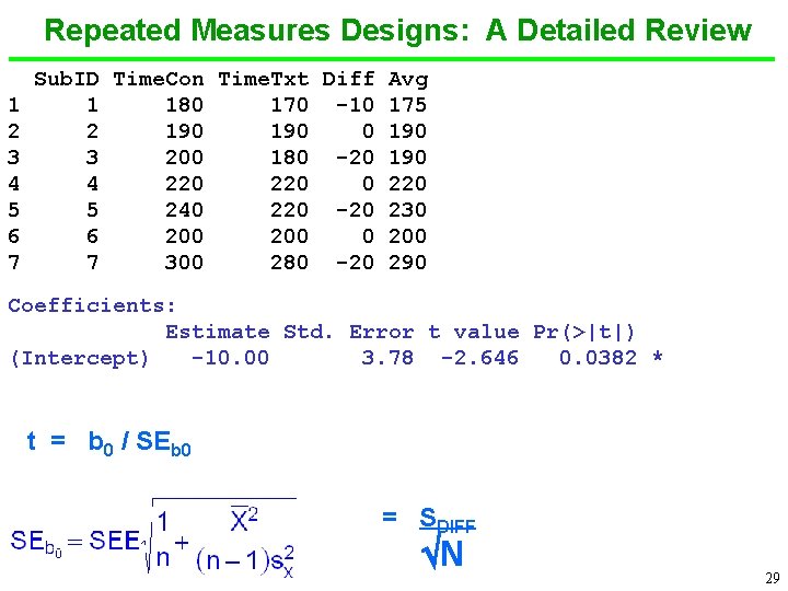
Repeated Measures Designs: A Detailed Review 1 2 3 4 5 6 7 Sub. ID Time. Con Time. Txt Diff Avg 1 180 170 -10 175 2 190 0 190 3 200 180 -20 190 4 220 0 220 5 240 220 -20 230 6 200 0 200 7 300 280 -20 290 d. W 1$Avg = (d. W 1$Time. Txt + d. W 1$Time. Con)/2 m. Avg = lm(Avg ~ 1, data=d. W 1) summary(m. Avg) #intercepts Coefficients: Estimate Std. Error t value Pr(>|t|) (Intercept) 213. 57 14. 59 14. 64 6. 37 e-06 *** The intercept of this model tests if the average marathon time is 0. Not an interesting question in this instance. 27

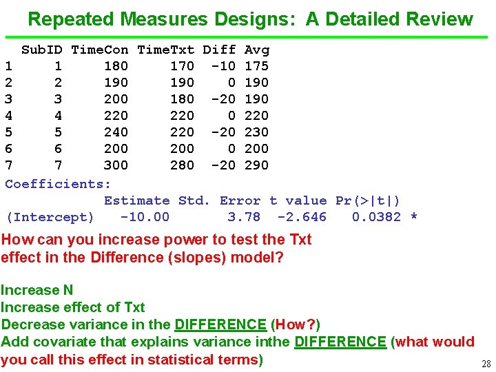
Repeated Measures Designs: A Detailed Review Sub. ID Time. Con Time. Txt Diff Avg 1 1 180 170 -10 175 2 2 190 0 190 3 3 200 180 -20 190 4 4 220 0 220 5 5 240 220 -20 230 6 6 200 0 200 7 7 300 280 -20 290 Coefficients: Estimate Std. Error t value Pr(>|t|) (Intercept) -10. 00 3. 78 -2. 646 0. 0382 * How can you increase power to test the Txt effect in the Difference (slopes) model? Increase N Increase effect of Txt Decrease variance in the DIFFERENCE (How? ) Add covariate that explains variance inthe DIFFERENCE (what would you call this effect in statistical terms) 28

Repeated Measures Designs: A Detailed Review 1 2 3 4 5 6 7 Sub. ID Time. Con Time. Txt Diff Avg 1 180 170 -10 175 2 190 0 190 3 200 180 -20 190 4 220 0 220 5 240 220 -20 230 6 200 0 200 7 300 280 -20 290 Coefficients: Estimate Std. Error t value Pr(>|t|) (Intercept) -10. 00 3. 78 -2. 646 0. 0382 * t = b 0 / SEb 0 = SDIFF N 29

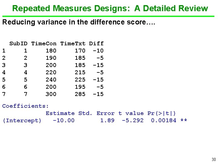
Repeated Measures Designs: A Detailed Review Reducing variance in the difference score…. 1 2 3 4 5 6 7 Sub. ID Time. Con Time. Txt Diff 1 180 170 -10 2 190 185 -5 3 200 185 -15 4 220 215 -5 5 240 225 -15 6 200 195 -5 7 300 285 -15 Coefficients: Estimate Std. Error t value Pr(>|t|) (Intercept) -10. 00 1. 89 -5. 292 0. 00184 ** 30

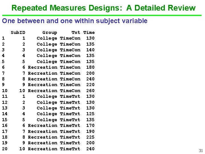
Repeated Measures Designs: A Detailed Review One between and one within subject variable 1 2 3 4 5 6 7 8 9 10 11 12 13 14 15 16 17 18 19 20 Sub. ID 1 2 3 4 5 6 7 8 9 10 Group College College College Recreation Recreation Recreation Txt Time. Con 130 Time. Con 135 Time. Con 140 Time. Con 135 Time. Con 180 Time. Con 200 Time. Con 240 Time. Con 220 Time. Con 260 Time. Txt 130 Time. Txt 125 Time. Txt 135 Time. Txt 170 Time. Txt 190 Time. Txt 225 Time. Txt 200 Time. Txt 240 31

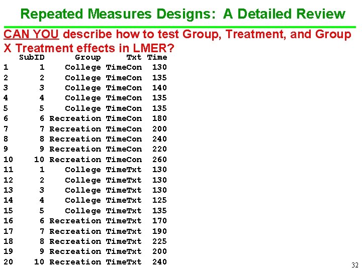
Repeated Measures Designs: A Detailed Review CAN YOU describe how to test Group, Treatment, and Group X Treatment effects in LMER? 1 2 3 4 5 6 7 8 9 10 11 12 13 14 15 16 17 18 19 20 Sub. ID 1 2 3 4 5 6 7 8 9 10 Group College College College Recreation Recreation Recreation Txt Time. Con 130 Time. Con 135 Time. Con 140 Time. Con 135 Time. Con 180 Time. Con 200 Time. Con 240 Time. Con 220 Time. Con 260 Time. Txt 130 Time. Txt 125 Time. Txt 135 Time. Txt 170 Time. Txt 190 Time. Txt 225 Time. Txt 200 Time. Txt 240 32

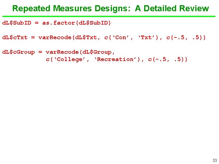
Repeated Measures Designs: A Detailed Review d. L$Sub. ID = as. factor(d. L$Sub. ID) d. L$c. Txt = var. Recode(d. L$Txt, c(‘Con’, ‘Txt’), c(-. 5, . 5)) d. L$c. Group = var. Recode(d. L$Group, c(‘College’, ‘Recreation’), c(-. 5, . 5)) 33

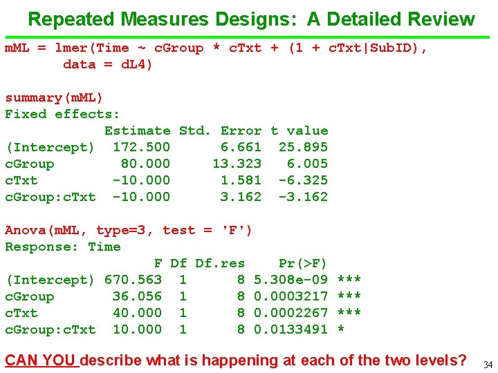
Repeated Measures Designs: A Detailed Review m. ML = lmer(Time ~ c. Group * c. Txt + (1 + c. Txt|Sub. ID), data = d. L 4) summary(m. ML) Fixed effects: Estimate Std. Error t value (Intercept) 172. 500 6. 661 25. 895 c. Group 80. 000 13. 323 6. 005 c. Txt -10. 000 1. 581 -6. 325 c. Group: c. Txt -10. 000 3. 162 -3. 162 Anova(m. ML, type=3, test = 'F') Response: Time F Df Df. res Pr(>F) (Intercept) 670. 563 1 8 5. 308 e-09 c. Group 36. 056 1 8 0. 0003217 c. Txt 40. 000 1 8 0. 0002267 c. Group: c. Txt 10. 000 1 8 0. 0133491 *** *** * CAN YOU describe what is happening at each of the two levels? 34

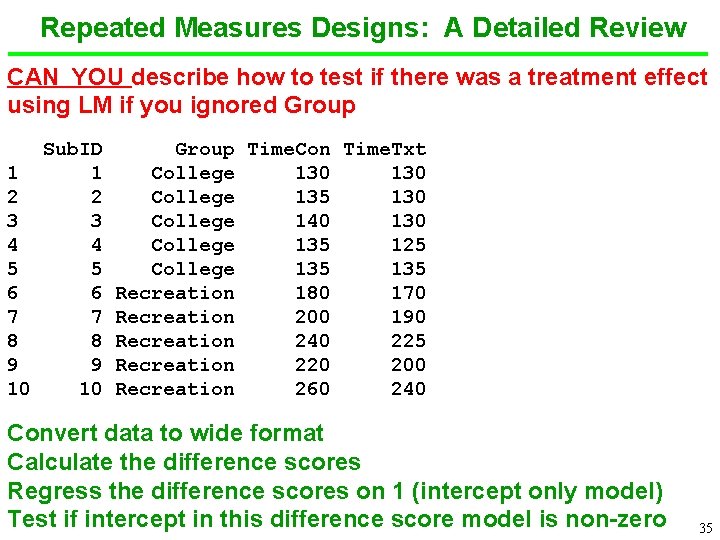
Repeated Measures Designs: A Detailed Review CAN YOU describe how to test if there was a treatment effect using LM if you ignored Group Sub. ID 1 1 2 2 3 3 4 4 5 5 6 6 7 7 8 8 9 9 10 10 Group Time. Con Time. Txt College 130 College 135 130 College 140 130 College 135 125 College 135 Recreation 180 170 Recreation 200 190 Recreation 240 225 Recreation 220 200 Recreation 260 240 Convert data to wide format Calculate the difference scores Regress the difference scores on 1 (intercept only model) Test if intercept in this difference score model is non-zero 35

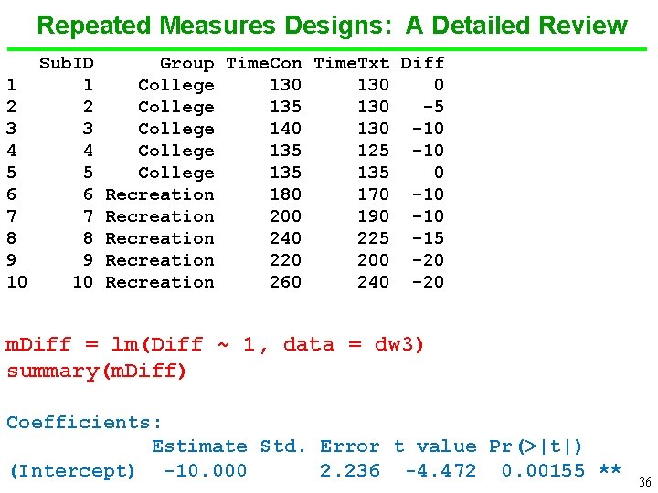
Repeated Measures Designs: A Detailed Review Sub. ID 1 1 2 2 3 3 4 4 5 5 6 6 7 7 8 8 9 9 10 10 Group Time. Con Time. Txt Diff College 130 0 College 135 130 -5 College 140 130 -10 College 135 125 -10 College 135 0 Recreation 180 170 -10 Recreation 200 190 -10 Recreation 240 225 -15 Recreation 220 200 -20 Recreation 260 240 -20 m. Diff = lm(Diff ~ 1, data = dw 3) summary(m. Diff) Coefficients: Estimate Std. Error t value Pr(>|t|) (Intercept) -10. 000 2. 236 -4. 472 0. 00155 ** 36

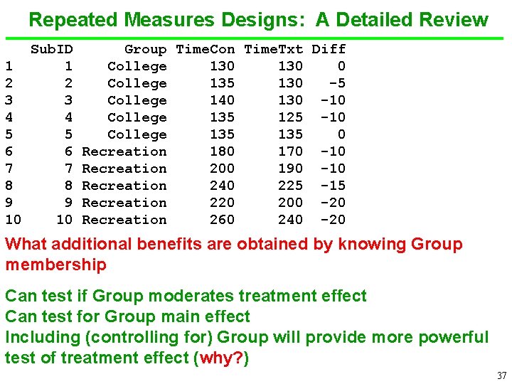
Repeated Measures Designs: A Detailed Review Sub. ID 1 1 2 2 3 3 4 4 5 5 6 6 7 7 8 8 9 9 10 10 Group Time. Con Time. Txt Diff College 130 0 College 135 130 -5 College 140 130 -10 College 135 125 -10 College 135 0 Recreation 180 170 -10 Recreation 200 190 -10 Recreation 240 225 -15 Recreation 220 200 -20 Recreation 260 240 -20 What additional benefits are obtained by knowing Group membership Can test if Group moderates treatment effect Can test for Group main effect Including (controlling for) Group will provide more powerful test of treatment effect (why? ) 37

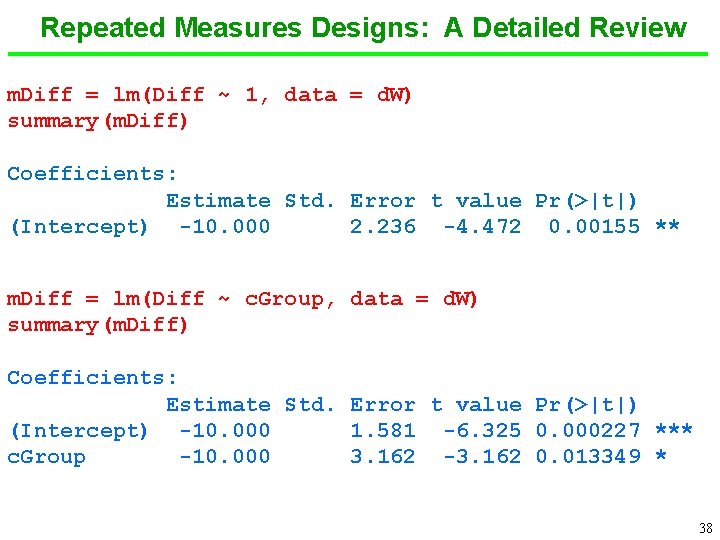
Repeated Measures Designs: A Detailed Review m. Diff = lm(Diff ~ 1, data = d. W) summary(m. Diff) Coefficients: Estimate Std. Error t value Pr(>|t|) (Intercept) -10. 000 2. 236 -4. 472 0. 00155 ** m. Diff = lm(Diff ~ c. Group, data = d. W) summary(m. Diff) Coefficients: Estimate Std. Error t value Pr(>|t|) (Intercept) -10. 000 1. 581 -6. 325 0. 000227 *** c. Group -10. 000 3. 162 -3. 162 0. 013349 * 38

And now on to new stuff…. . An Alternative Approach to Repeated Measures 39 39

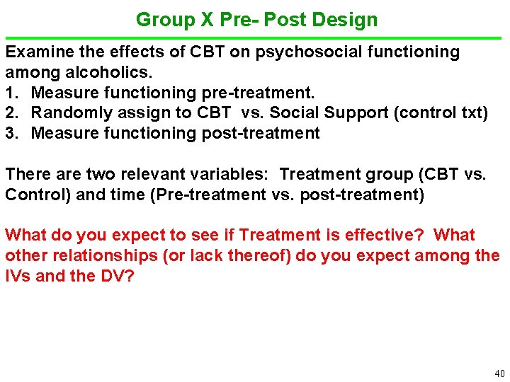
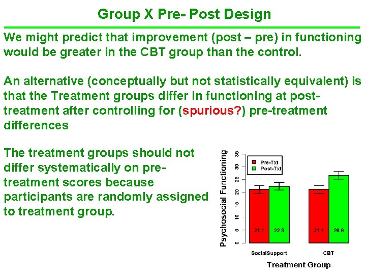
Group X Pre- Post Design Examine the effects of CBT on psychosocial functioning among alcoholics. 1. Measure functioning pre-treatment. 2. Randomly assign to CBT vs. Social Support (control txt) 3. Measure functioning post-treatment There are two relevant variables: Treatment group (CBT vs. Control) and time (Pre-treatment vs. post-treatment) What do you expect to see if Treatment is effective? What other relationships (or lack thereof) do you expect among the IVs and the DV? 40 40

Group X Pre- Post Design We might predict that improvement (post – pre) in functioning would be greater in the CBT group than the control. An alternative (conceptually but not statistically equivalent) is that the Treatment groups differ in functioning at posttreatment after controlling for (spurious? ) pre-treatment differences The treatment groups should not differ systematically on pretreatment scores because participants are randomly assigned to treatment group. 41 41

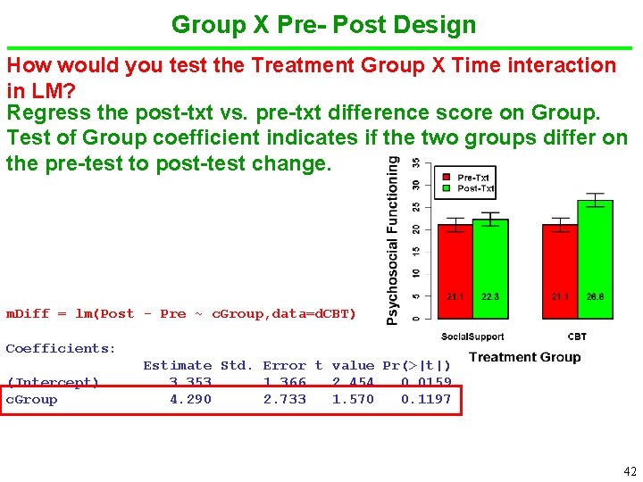
Group X Pre- Post Design How would you test the Treatment Group X Time interaction in LM? Regress the post-txt vs. pre-txt difference score on Group. Test of Group coefficient indicates if the two groups differ on the pre-test to post-test change. m. Diff = lm(Post - Pre ~ c. Group, data=d. CBT) Coefficients: (Intercept) c. Group Estimate Std. Error t value Pr(>|t|) 3. 353 1. 366 2. 454 0. 0159 4. 290 2. 733 1. 570 0. 1197 42 42

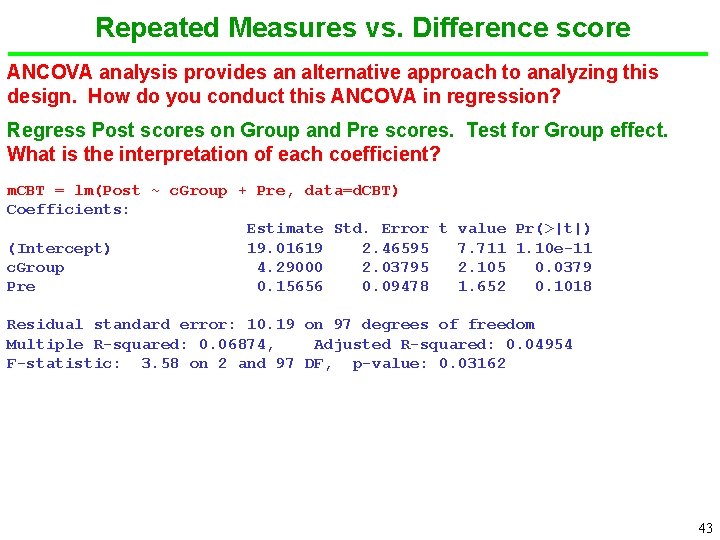
Repeated Measures vs. Difference score ANCOVA analysis provides an alternative approach to analyzing this design. How do you conduct this ANCOVA in regression? Regress Post scores on Group and Pre scores. Test for Group effect. What is the interpretation of each coefficient? m. CBT = lm(Post ~ c. Group + Pre, data=d. CBT) Coefficients: Estimate Std. Error t value Pr(>|t|) (Intercept) 19. 01619 2. 46595 7. 711 1. 10 e-11 c. Group 4. 29000 2. 03795 2. 105 0. 0379 Pre 0. 15656 0. 09478 1. 652 0. 1018 Residual standard error: 10. 19 on 97 degrees of freedom Multiple R-squared: 0. 06874, Adjusted R-squared: 0. 04954 F-statistic: 3. 58 on 2 and 97 DF, p-value: 0. 03162 43 43

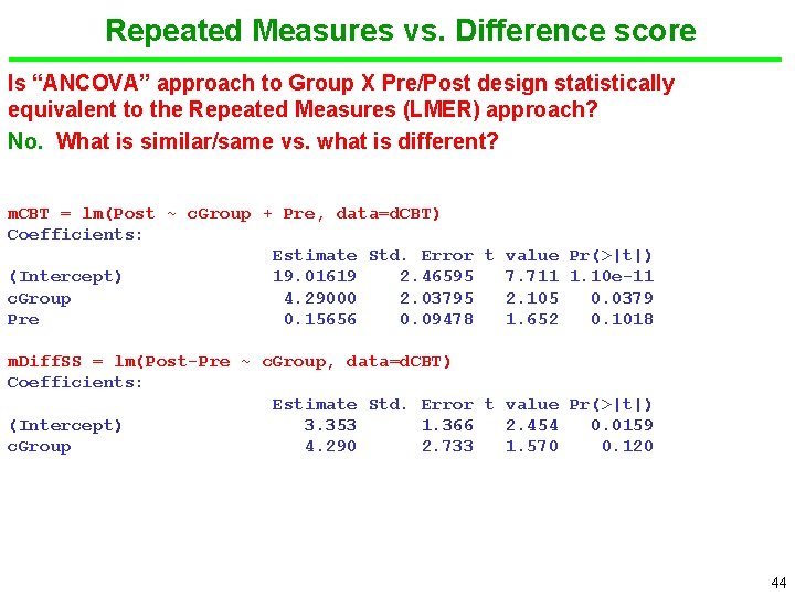
Repeated Measures vs. Difference score Is “ANCOVA” approach to Group X Pre/Post design statistically equivalent to the Repeated Measures (LMER) approach? No. What is similar/same vs. what is different? m. CBT = lm(Post ~ c. Group + Pre, data=d. CBT) Coefficients: Estimate Std. Error t value Pr(>|t|) (Intercept) 19. 01619 2. 46595 7. 711 1. 10 e-11 c. Group 4. 29000 2. 03795 2. 105 0. 0379 Pre 0. 15656 0. 09478 1. 652 0. 1018 m. Diff. SS = lm(Post-Pre ~ c. Group, data=d. CBT) Coefficients: Estimate Std. Error t value Pr(>|t|) (Intercept) 3. 353 1. 366 2. 454 0. 0159 c. Group 4. 290 2. 733 1. 570 0. 120 44 44

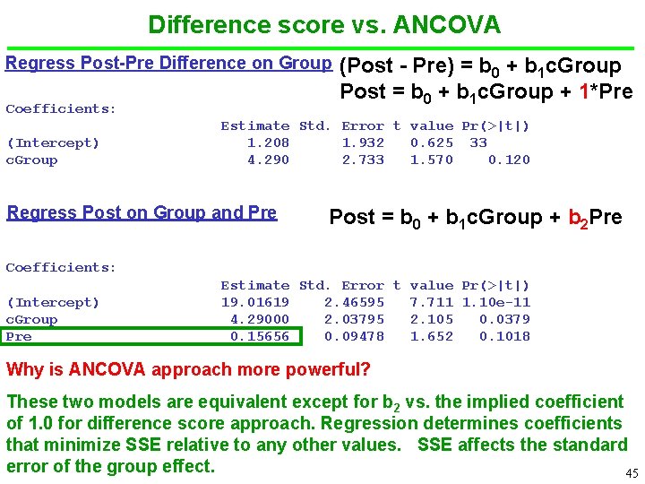
Difference score vs. ANCOVA Regress Post-Pre Difference on Group Coefficients: (Intercept) c. Group (Post - Pre) = b 0 + b 1 c. Group Post = b 0 + b 1 c. Group + 1*Pre Estimate Std. Error t value Pr(>|t|) 1. 208 1. 932 0. 625 33 4. 290 2. 733 1. 570 0. 120 Regress Post on Group and Pre Post = b 0 + b 1 c. Group + b 2 Pre Coefficients: (Intercept) c. Group Pre Estimate Std. Error t value Pr(>|t|) 19. 01619 2. 46595 7. 711 1. 10 e-11 4. 29000 2. 03795 2. 105 0. 0379 0. 15656 0. 09478 1. 652 0. 1018 Why is ANCOVA approach more powerful? These two models are equivalent except for b 2 vs. the implied coefficient of 1. 0 for difference score approach. Regression determines coefficients that minimize SSE relative to any other values. SSE affects the standard 45 error of the group effect. 45

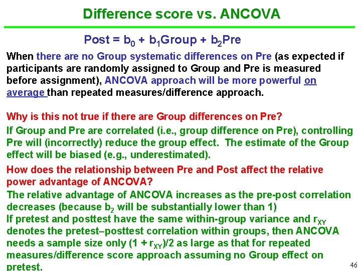
Difference score vs. ANCOVA Post = b 0 + b 1 Group + b 2 Pre When there are no Group systematic differences on Pre (as expected if participants are randomly assigned to Group and Pre is measured before assignment), ANCOVA approach will be more powerful on average than repeated measures/difference approach. Why is this not true if there are Group differences on Pre? If Group and Pre are correlated (i. e. , group difference on Pre), controlling Pre will (incorrectly) reduce the group effect. The estimate of the Group effect will be biased (e. g. , underestimated). How does the relationship between Pre and Post affect the relative power advantage of ANCOVA? The relative advantage of ANCOVA increases as the pre-post correlation decreases (because b 2 will be substantially lower than 1) If pretest and posttest have the same within-group variance and r. XY denotes the pretest–posttest correlation within groups, then ANCOVA needs a sample size only (1 + r. XY)/2 as large as that for repeated measures/difference score approach assuming no Group effect on 46 46 pretest.

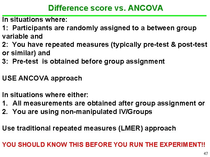
Difference score vs. ANCOVA In situations where: 1: Participants are randomly assigned to a between group variable and 2: You have repeated measures (typically pre-test & post-test or similar) and 3: Pre-test is obtained before group assignment USE ANCOVA approach In situations where either: 1. All measurements are obtained after group assignment or 2. You are using non-manipulated IV/Groups Use traditional repeated measures (LMER) approach YOU SHOULD KNOW THIS BEFORE YOU RUN THE EXPERIMENT!! 47