Unit 1 Trade Theory Specific Factors Model 212012

Unit 1: Trade Theory Specific Factors Model 2/1/2012

Definitions specific factor – factor that can only be used in the production of a particular good mobile factor – factor that can move between sectors

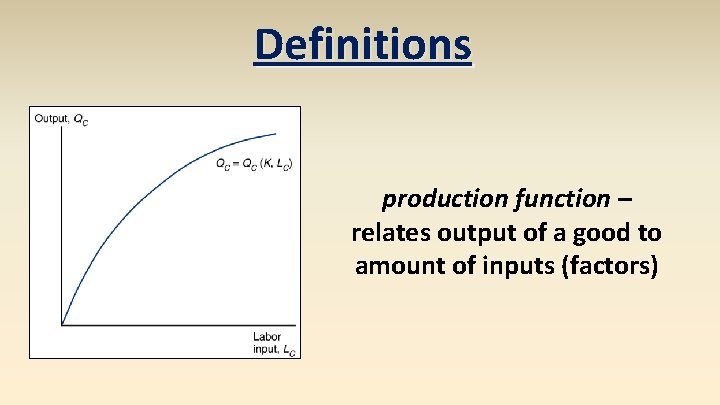
Definitions production function – relates output of a good to amount of inputs (factors)

Definitions marginal product of labor – addition to output generated by adding 1 person hour

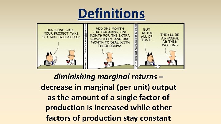
Definitions diminishing marginal returns – decrease in marginal (per unit) output as the amount of a single factor of production is increased while other factors of production stay constant

Definitions budget constraint – combinations of goods available for consumption given an income

capital owners Definitions workers income distribution – division of revenues among factors of production landowners

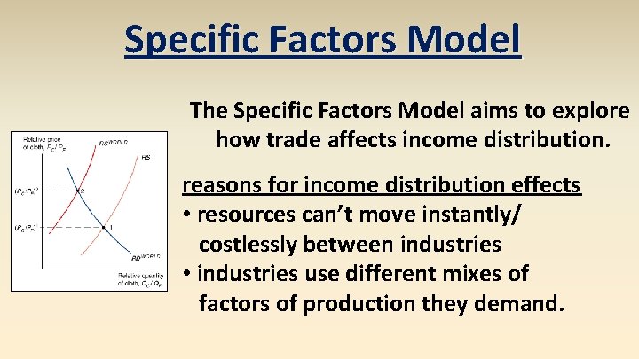
Specific Factors Model The Specific Factors Model aims to explore how trade affects income distribution. reasons for income distribution effects • resources can’t move instantly/ costlessly between industries • industries use different mixes of factors of production they demand.

Specific Factors: assumptions 1. 2. 3. 4. 5. 6. 2 goods: cloth & food. 3 factors of production: labor (L), capital (K), & land (T). Perfect competition in all markets. Cloth produced using capital and labor (not land). Food produced using land labor (not capital). Labor is a mobile factor. • can move between sectors 7. Land capital are both specific factors. • used only in the production of one good

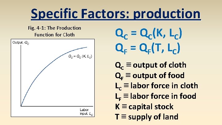
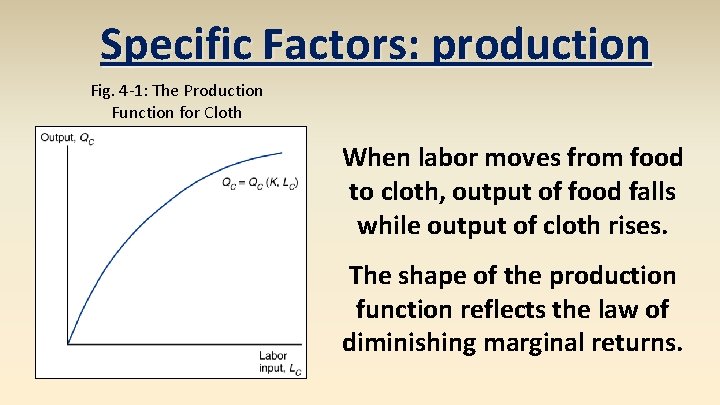
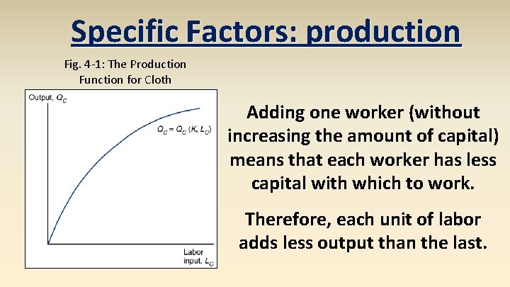
Specific Factors: production Fig. 4 -1: The Production Function for Cloth QC = QC(K, LC) QF = QF(T, LC) QC ≡ output of cloth QF ≡ output of food LC ≡ labor force in cloth LF ≡ labor force in food K ≡ capital stock T ≡ supply of land

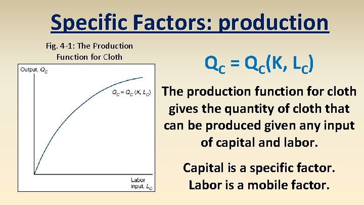
Specific Factors: production Fig. 4 -1: The Production Function for Cloth QC = QC(K, LC) The production function for cloth gives the quantity of cloth that can be produced given any input of capital and labor. Capital is a specific factor. Labor is a mobile factor.

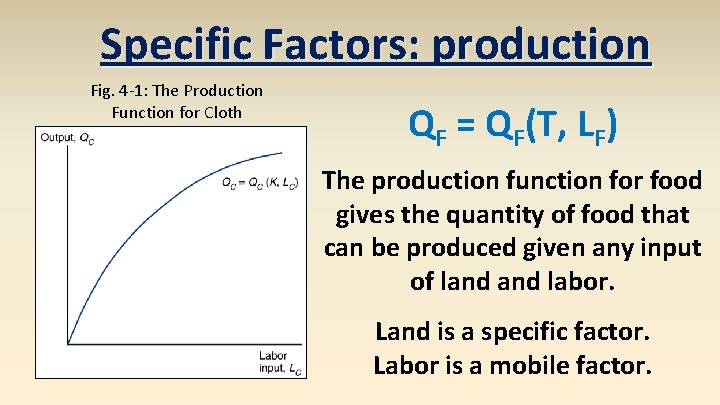
Specific Factors: production Fig. 4 -1: The Production Function for Cloth QF = QF(T, LF) The production function for food gives the quantity of food that can be produced given any input of land labor. Land is a specific factor. Labor is a mobile factor.

Specific Factors: production Fig. 4 -1: The Production Function for Cloth When labor moves from food to cloth, output of food falls while output of cloth rises. The shape of the production function reflects the law of diminishing marginal returns.

Specific Factors: production diminishing marginal returns – decrease in marginal (per unit) output as the amount of a single factor of production is increased while other factors of production stay constant

Specific Factors: production Fig. 4 -1: The Production Function for Cloth Adding one worker (without increasing the amount of capital) means that each worker has less capital with which to work. Therefore, each unit of labor adds less output than the last.

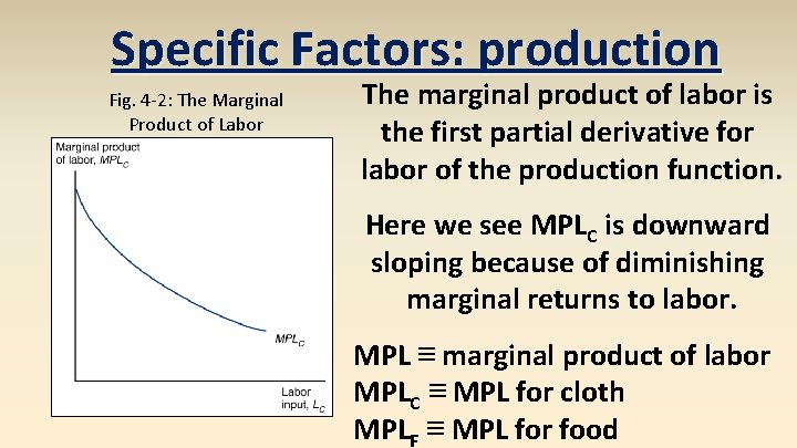
Specific Factors: production Fig. 4 -2: The Marginal Product of Labor The marginal product of labor is the first partial derivative for labor of the production function. Here we see MPLC is downward sloping because of diminishing marginal returns to labor. MPL ≡ marginal product of labor MPLC ≡ MPL for cloth MPLF ≡ MPL for food

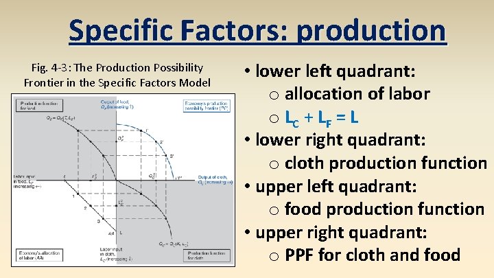
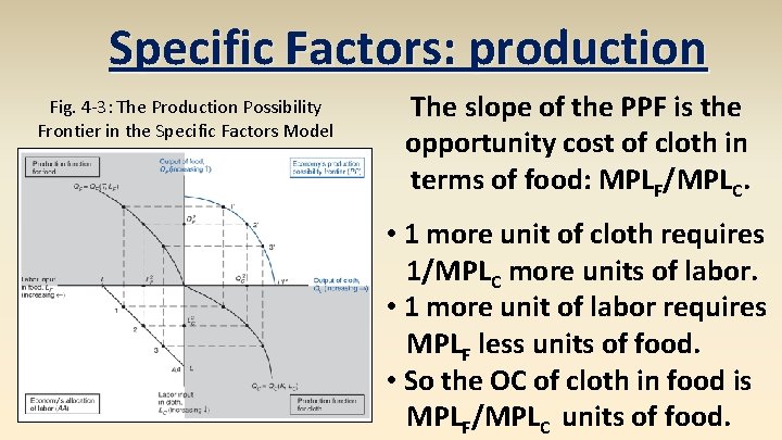
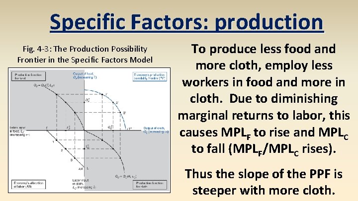
Specific Factors: production Fig. 4 -3: The Production Possibility Frontier in the Specific Factors Model Here we see the production possibilities frontier (PPF) derived using a 4 quadrant diagram. This shows how diminishing marginal returns to labor leads to a curved PPF. Follow the dotted lines from points on the allocation of labor line to the PPF.

Specific Factors: production Fig. 4 -3: The Production Possibility Frontier in the Specific Factors Model • lower left quadrant: o allocation of labor o LC + LF = L • lower right quadrant: o cloth production function • upper left quadrant: o food production function • upper right quadrant: o PPF for cloth and food

Specific Factors: production Fig. 4 -3: The Production Possibility Frontier in the Specific Factors Model The slope of the PPF is the opportunity cost of cloth in terms of food: MPLF/MPLC. • 1 more unit of cloth requires 1/MPLC more units of labor. • 1 more unit of labor requires MPLF less units of food. • So the OC of cloth in food is MPLF/MPLC units of food.

Specific Factors: production Fig. 4 -3: The Production Possibility Frontier in the Specific Factors Model To produce less food and more cloth, employ less workers in food and more in cloth. Due to diminishing marginal returns to labor, this causes MPLF to rise and MPLC to fall (MPLF/MPLC rises). Thus the slope of the PPF is steeper with more cloth.

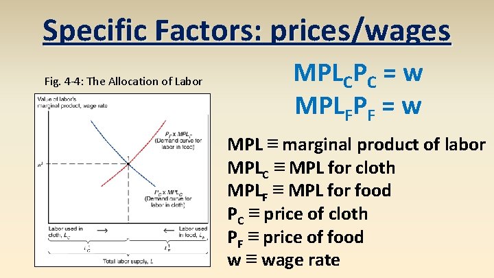
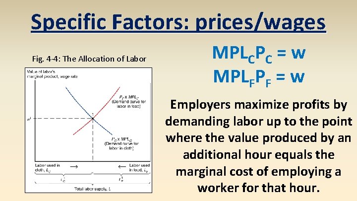
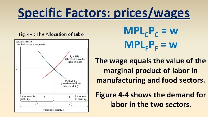
Specific Factors: prices/wages Fig. 4 -4: The Allocation of Labor MPLCPC = w MPLFPF = w MPL ≡ marginal product of labor MPLC ≡ MPL for cloth MPLF ≡ MPL for food PC ≡ price of cloth PF ≡ price of food w ≡ wage rate

Specific Factors: prices/wages Fig. 4 -4: The Allocation of Labor MPLCPC = w MPLFPF = w Employers maximize profits by demanding labor up to the point where the value produced by an additional hour equals the marginal cost of employing a worker for that hour.

Specific Factors: prices/wages Fig. 4 -4: The Allocation of Labor MPLCPC = w MPLFPF = w The wage equals the value of the marginal product of labor in manufacturing and food sectors. Figure 4 -4 shows the demand for labor in the two sectors.

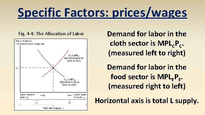
Specific Factors: prices/wages Fig. 4 -4: The Allocation of Labor Demand for labor in the cloth sector is MPLCPC. (measured left to right) Demand for labor in the food sector is MPLFPF. (measured right to left) Horizontal axis is total L supply.

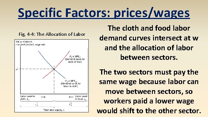
Specific Factors: prices/wages Fig. 4 -4: The Allocation of Labor The cloth and food labor demand curves intersect at w and the allocation of labor between sectors. The two sectors must pay the same wage because labor can move between sectors, so workers paid a lower wage would shift to the other sector.

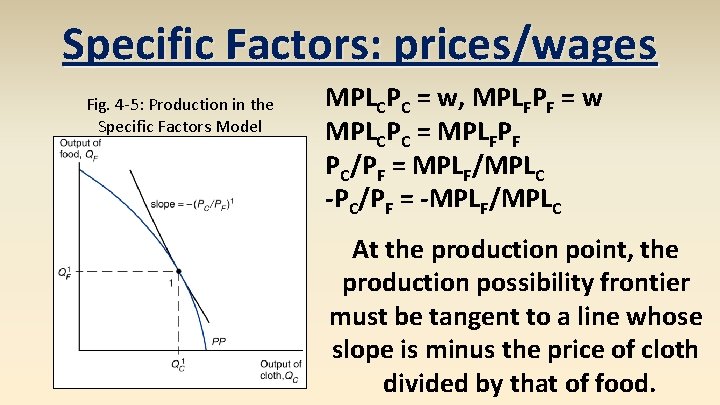
Specific Factors: prices/wages Fig. 4 -5: Production in the Specific Factors Model MPLCPC = w, MPLFPF = w MPLCPC = MPLFPF PC/PF = MPLF/MPLC -PC/PF = -MPLF/MPLC At the production point, the production possibility frontier must be tangent to a line whose slope is minus the price of cloth divided by that of food.

Specific Factors: income dist. What happens to the allocation of labor and the distribution of income when the prices of food and cloth change? 2 cases • equal (proportional) change • change in relative prices

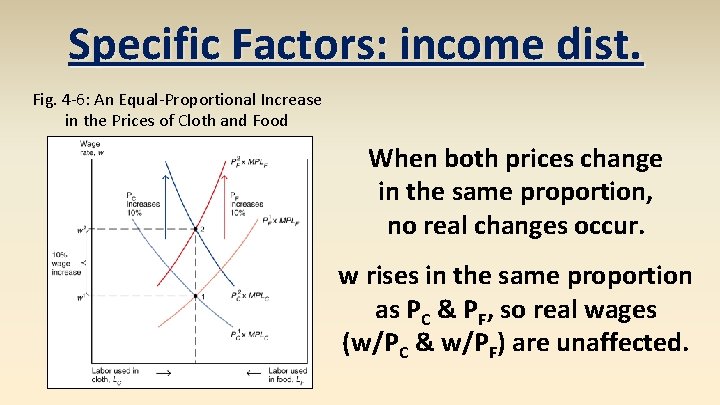
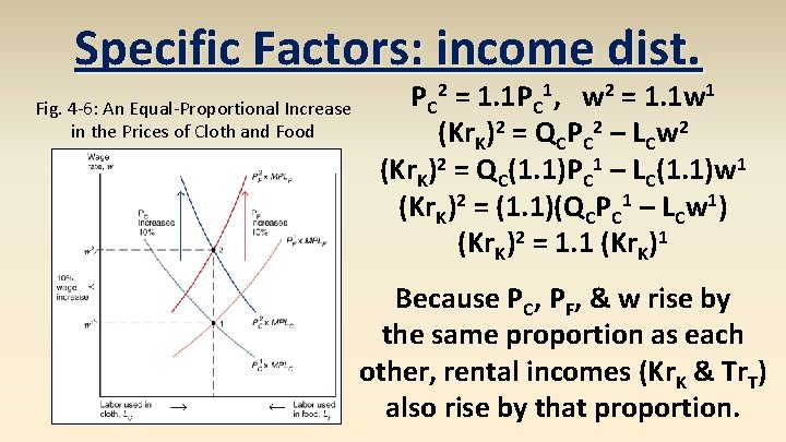
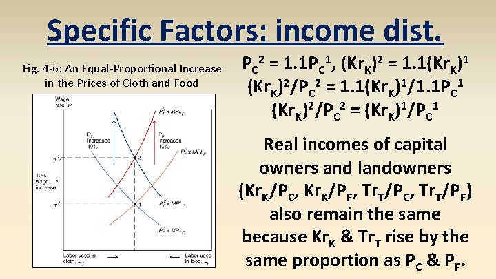
Specific Factors: income dist. Fig. 4 -6: An Equal-Proportional Increase in the Prices of Cloth and Food When both prices change in the same proportion, no real changes occur. w rises in the same proportion as PC & PF, so real wages (w/PC & w/PF) are unaffected.

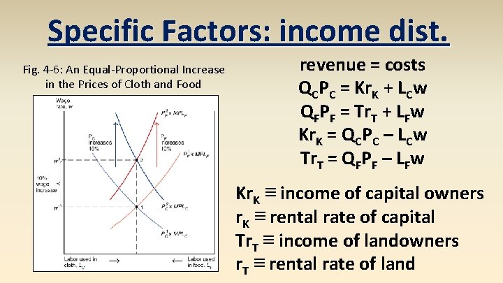
Specific Factors: income dist. Fig. 4 -6: An Equal-Proportional Increase in the Prices of Cloth and Food revenue = costs QCPC = Kr. K + LCw QFPF = Tr. T + LFw Kr. K = QCPC – LCw Tr. T = QFPF – LFw Kr. K ≡ income of capital owners r. K ≡ rental rate of capital Tr. T ≡ income of landowners r. T ≡ rental rate of land

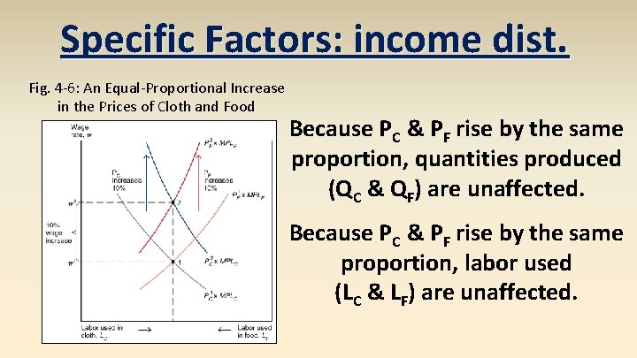
Specific Factors: income dist. Fig. 4 -6: An Equal-Proportional Increase in the Prices of Cloth and Food Because PC & PF rise by the same proportion, quantities produced (QC & QF) are unaffected. Because PC & PF rise by the same proportion, labor used (LC & LF) are unaffected.

Specific Factors: income dist. Fig. 4 -6: An Equal-Proportional Increase in the Prices of Cloth and Food PC 2 = 1. 1 PC 1, w 2 = 1. 1 w 1 (Kr. K)2 = QCPC 2 – LCw 2 (Kr. K)2 = QC(1. 1)PC 1 – LC(1. 1)w 1 (Kr. K)2 = (1. 1)(QCPC 1 – LCw 1) (Kr. K)2 = 1. 1 (Kr. K)1 Because PC, PF, & w rise by the same proportion as each other, rental incomes (Kr. K & Tr. T) also rise by that proportion.

Specific Factors: income dist. Fig. 4 -6: An Equal-Proportional Increase in the Prices of Cloth and Food PC 2 = 1. 1 PC 1, (Kr. K)2 = 1. 1(Kr. K)1 (Kr. K)2/PC 2 = 1. 1(Kr. K)1/1. 1 PC 1 (Kr. K)2/PC 2 = (Kr. K)1/PC 1 Real incomes of capital owners and landowners (Kr. K/PC, Kr. K/PF, Tr. T/PC, Tr. T/PF) also remain the same because Kr. K & Tr. T rise by the same proportion as PC & PF.

Specific Factors: income dist. capital owners workers Thus when both prices change in the same proportion, no real changes occur. The real incomes of workers, capital owners, and landowners are unaffected. landowners

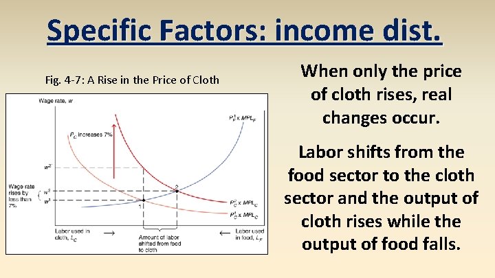
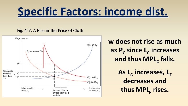
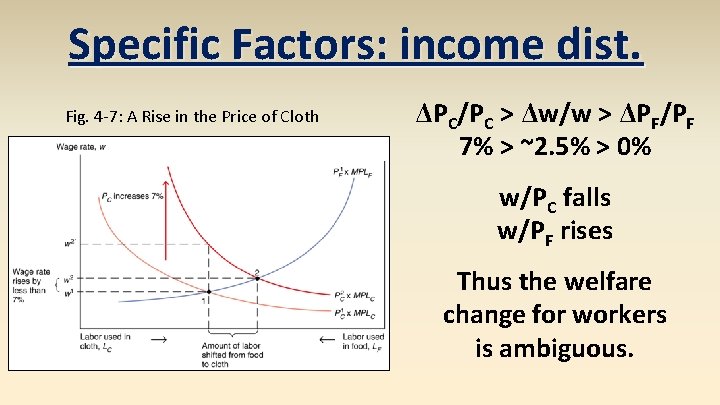
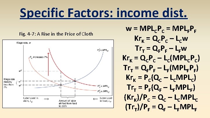
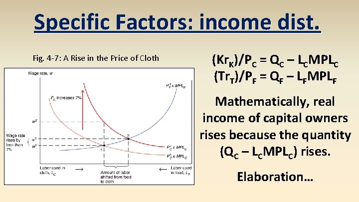
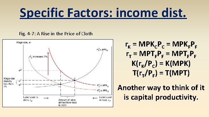
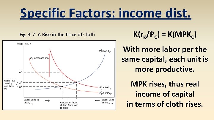
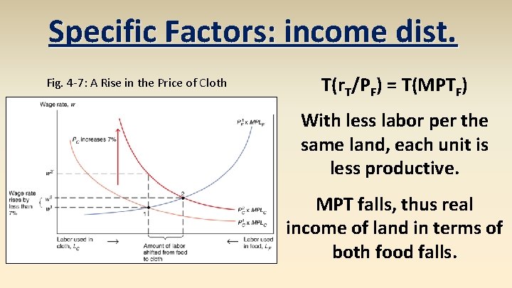
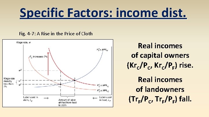
Specific Factors: income dist. Fig. 4 -7: A Rise in the Price of Cloth When only the price of cloth rises, real changes occur. Labor shifts from the food sector to the cloth sector and the output of cloth rises while the output of food falls.

Specific Factors: income dist. Fig. 4 -7: A Rise in the Price of Cloth w does not rise as much as PC since LC increases and thus MPLC falls. As LC increases, LF decreases and thus MPLF rises.

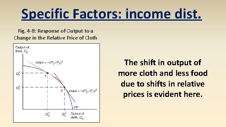
Specific Factors: income dist. Fig. 4 -8: Response of Output to a Change in the Relative Price of Cloth The shift in output of more cloth and less food due to shifts in relative prices is evident here.

Specific Factors: income dist. Fig. 4 -7: A Rise in the Price of Cloth ΔPC/PC > Δw/w > ΔPF/PF 7% > ~2. 5% > 0% w/PC falls w/PF rises Thus the welfare change for workers is ambiguous.

Specific Factors: income dist. Fig. 4 -7: A Rise in the Price of Cloth w = MPLCPC = MPLFPF Kr. K = QCPC – LCw Tr. T = QFPF – LFw Kr. K = QCPC – LC(MPLCPC) Tr. T = QFPF – LF(MPLFPF) Kr. K = PC(QC – LCMPLC) Tr. T = PF(QF – LFMPLF) (Kr. K)/PC = QC – LCMPLC (Tr. T)/PF = QF – LFMPLF

Specific Factors: income dist. Fig. 4 -7: A Rise in the Price of Cloth (Kr. K)/PC = QC – LCMPLC (Tr. T)/PF = QF – LFMPLF Mathematically, real income of capital owners rises because the quantity (QC – LCMPLC) rises. Elaboration…

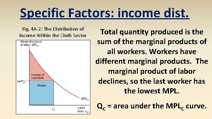
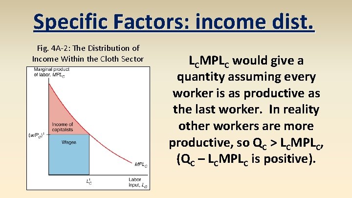
Specific Factors: income dist. Fig. 4 A-2: The Distribution of Income Within the Cloth Sector Total quantity produced is the sum of the marginal products of all workers. Workers have different marginal products. The marginal product of labor declines, so the last worker has the lowest MPL. QC = area under the MPLC curve.

Specific Factors: income dist. Fig. 4 A-2: The Distribution of Income Within the Cloth Sector LCMPLC would give a quantity assuming every worker is as productive as the last worker. In reality other workers are more productive, so QC > LCMPLC, (QC – LCMPLC is positive).

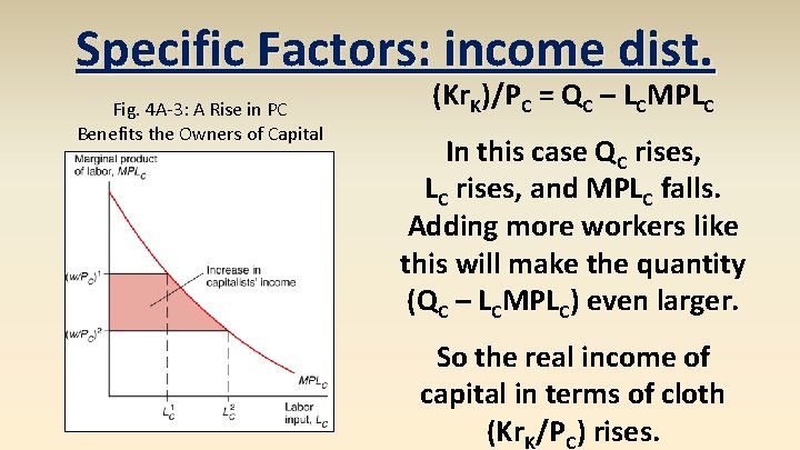
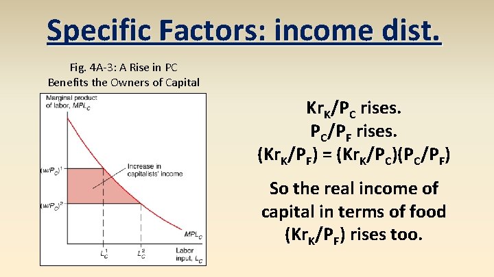
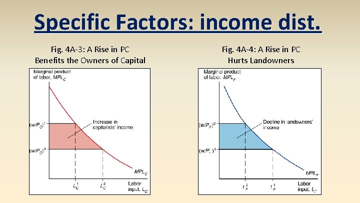
Specific Factors: income dist. Fig. 4 A-3: A Rise in PC Benefits the Owners of Capital (Kr. K)/PC = QC – LCMPLC In this case QC rises, LC rises, and MPLC falls. Adding more workers like this will make the quantity (QC – LCMPLC) even larger. So the real income of capital in terms of cloth (Kr. K/PC) rises.

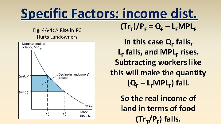
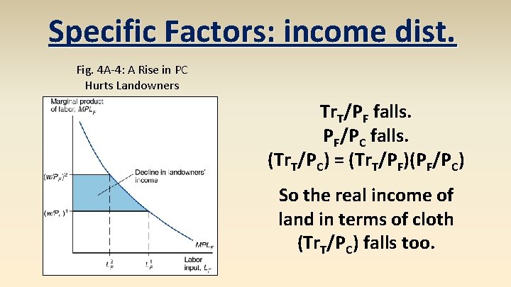
Specific Factors: income dist. Fig. 4 A-4: A Rise in PC Hurts Landowners (Tr. T)/PF = QF – LFMPLF In this case QF falls, LF falls, and MPLF rises. Subtracting workers like this will make the quantity (QF – LFMPLF) fall. So the real income of land in terms of food (Tr. T/PF) falls.

Specific Factors: income dist. Fig. 4 A-3: A Rise in PC Benefits the Owners of Capital Kr. K/PC rises. PC/PF rises. (Kr. K/PF) = (Kr. K/PC)(PC/PF) So the real income of capital in terms of food (Kr. K/PF) rises too.

Specific Factors: income dist. Fig. 4 A-4: A Rise in PC Hurts Landowners Tr. T/PF falls. PF/PC falls. (Tr. T/PC) = (Tr. T/PF)(PF/PC) So the real income of land in terms of cloth (Tr. T/PC) falls too.

Specific Factors: income dist. Fig. 4 A-2: The Distribution of Income Within the Cloth Sector Changes in income of capital owners and landowners are easier to see graphically as consumer surpluses on the MPL curves.

Specific Factors: income dist. Fig. 4 A-3: A Rise in PC Benefits the Owners of Capital Fig. 4 A-4: A Rise in PC Hurts Landowners

Specific Factors: income dist. Fig. 4 -7: A Rise in the Price of Cloth r. K = MPKCPC = MPKFPF r. T = MPTFPF K(r. K/PC) = K(MPK) T(r. T/PF) = T(MPT) Another way to think of it is capital productivity.

Specific Factors: income dist. Fig. 4 -7: A Rise in the Price of Cloth K(r. K/PC) = K(MPKC) With more labor per the same capital, each unit is more productive. MPK rises, thus real income of capital in terms of cloth rises.

Specific Factors: income dist. Fig. 4 -7: A Rise in the Price of Cloth T(r. T/PF) = T(MPTF) With less labor per the same land, each unit is less productive. MPT falls, thus real income of land in terms of both food falls.

Specific Factors: income dist. Fig. 4 -7: A Rise in the Price of Cloth Real incomes of capital owners (Kr. C/PC, Kr. C/PF) rise. Real incomes of landowners (Tr. F/PC, Tr. F/PF) fall.

Specific Factors: income dist. capital owners workers landowners Thus when only the price of cloth rises, real changes occur. Capital owners are better off, landowners are worse off, and the welfare change of workers is ambiguous.

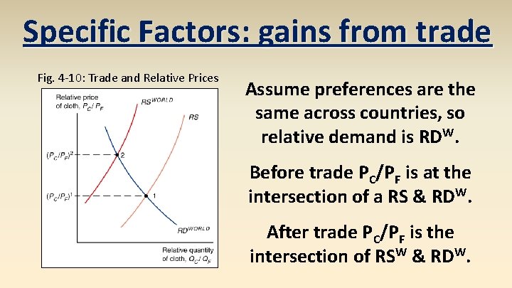
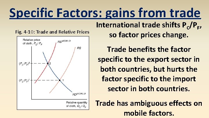
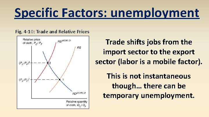
Specific Factors: gains from trade Fig. 4 -10: Trade and Relative Prices Assume preferences are the same across countries, so relative demand is RDW. Before trade PC/PF is at the intersection of a RS & RDW. After trade PC/PF is the intersection of RSW & RDW.

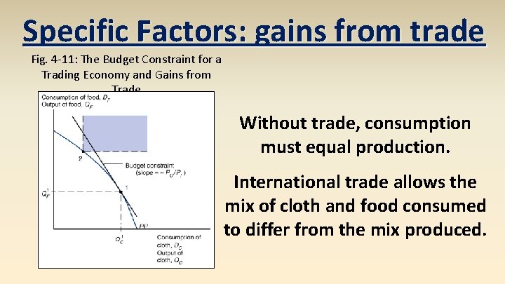
Specific Factors: gains from trade Fig. 4 -11: The Budget Constraint for a Trading Economy and Gains from Trade Without trade, consumption must equal production. International trade allows the mix of cloth and food consumed to differ from the mix produced.

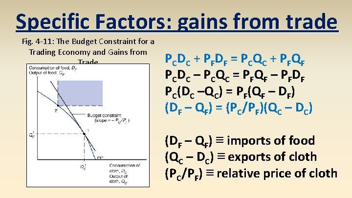
Specific Factors: gains from trade Fig. 4 -11: The Budget Constraint for a Trading Economy and Gains from Trade Budget constraint P C D C + P F D F = P C QC + P F QF PC ≡ price of cloth PF ≡ price of food DC ≡ cloth consumed DF ≡ food consumed QC ≡ cloth produced QF ≡ food produced

Specific Factors: gains from trade Fig. 4 -11: The Budget Constraint for a Trading Economy and Gains from Trade P C D C + P F D F = P C QC + P F QF P C D C – P C QC = P F QF – P F D F PC(DC –QC) = PF(QF – DF) (DF – QF) = (PC/PF)(QC – DC) (DF – QF) ≡ imports of food (QC – DC) ≡ exports of cloth (PC/PF) ≡ relative price of cloth

Specific Factors: gains from trade Fig. 4 -11: The Budget Constraint for a Trading Economy and Gains from Trade Country can afford amounts of cloth and food it can’t produce. Budget constraint with trade lies above the production possibilities frontier.

Specific Factors: gains from trade Fig. 4 -10: Trade and Relative Prices International trade shifts PC/PF, so factor prices change. Trade benefits the factor specific to the export sector in both countries, but hurts the factor specific to the import sector in both countries. Trade has ambiguous effects on mobile factors.

Specific Factors: gains from trade capital owners workers It is possible to redistribute income so that everyone gains. Those who gain from trade could compensate those who lose and still be better off. landowners Possible doesn’t mean it happens… hard to implement.

Specific Factors: political economy capital owners workers Trade produces both winners and losers. In spite of these income distribution effects, economists overwhelmingly favor free trade policies. Why? landowners 3 main reasons…

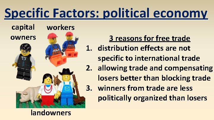
Specific Factors: political economy capital owners workers landowners 3 reasons for free trade 1. distribution effects are not specific to international trade 2. allowing trade and compensating losers better than blocking trade 3. winners from trade are less politically organized than losers

Specific Factors: political economy capital owners workers landowners There are winners and losers in all trade – not just international trade. Every change in the economy, including shifting consumer preferences and technology advances, helps some and hurts others. So don’t focus on distribution.

Specific Factors: political economy capital owners workers landowners If the government is going to intervene, it is better to compensate the losers than to block all trade. This preserves more of the gains for society than blocking trade would.

Specific Factors: political economy capital owners workers landowners Those who gain from trade are typically less concentrated, informed, and organized than those who lose. Losers can convince politicians to block trade with tariffs and quotas. As a counterweight, should favor free trade in general.

Specific Factors: unemployment Fig. 4 -10: Trade and Relative Prices Trade shifts jobs from the import sector to the export sector (labor is a mobile factor). This is not instantaneous though… there can be temporary unemployment.

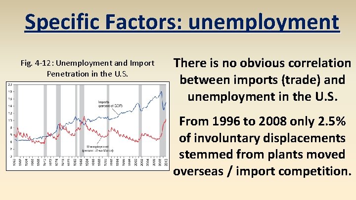
Specific Factors: unemployment Fig. 4 -12: Unemployment and Import Penetration in the U. S. There is no obvious correlation between imports (trade) and unemployment in the U. S. From 1996 to 2008 only 2. 5% of involuntary displacements stemmed from plants moved overseas / import competition.

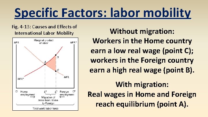
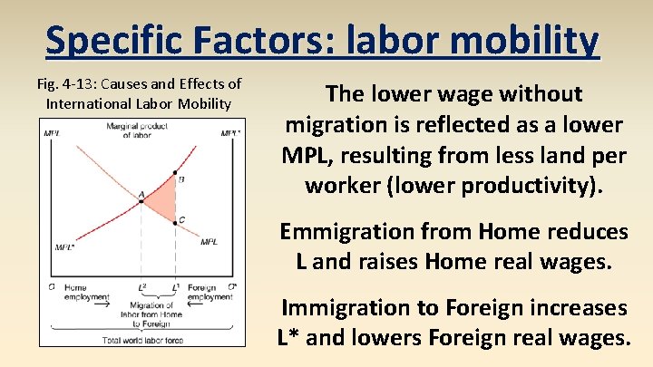
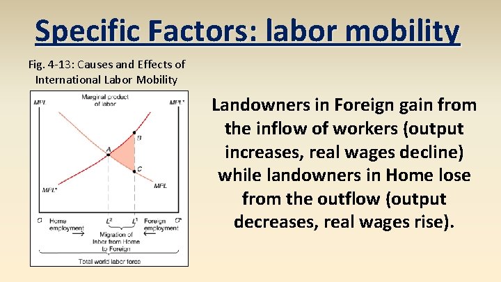
Specific Factors: labor mobility Fig. 4 -13: Causes and Effects of International Labor Mobility Workers migrate to where wages are highest. Suppose 2 countries produce a non-traded good (food) using a mobile factor (labor) and a specific factor (land).

Specific Factors: labor mobility Fig. 4 -13: Causes and Effects of International Labor Mobility Without migration: Workers in the Home country earn a low real wage (point C); workers in the Foreign country earn a high real wage (point B). With migration: Real wages in Home and Foreign reach equilibrium (point A).

Specific Factors: labor mobility Fig. 4 -13: Causes and Effects of International Labor Mobility The lower wage without migration is reflected as a lower MPL, resulting from less land per worker (lower productivity). Emmigration from Home reduces L and raises Home real wages. Immigration to Foreign increases L* and lowers Foreign real wages.

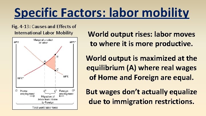
Specific Factors: labor mobility Fig. 4 -13: Causes and Effects of International Labor Mobility World output rises: labor moves to where it is more productive. Foreign gains the area under the trapezoid ABL 1 L 2. Home loses the area under the trapezoid ACL 1 L 2. Thus total output increases by the triangle ABC.

Specific Factors: labor mobility Fig. 4 -13: Causes and Effects of International Labor Mobility World output rises: labor moves to where it is more productive. World output is maximized at the equilibrium (A) where real wages of Home and Foreign are equal. But wages don’t actually equalize due to immigration restrictions.

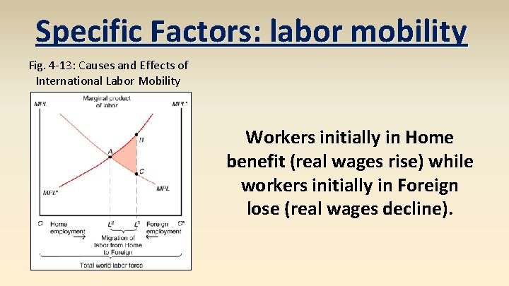
Specific Factors: labor mobility Fig. 4 -13: Causes and Effects of International Labor Mobility Workers initially in Home benefit (real wages rise) while workers initially in Foreign lose (real wages decline).

Specific Factors: labor mobility Fig. 4 -13: Causes and Effects of International Labor Mobility Landowners in Foreign gain from the inflow of workers (output increases, real wages decline) while landowners in Home lose from the outflow (output decreases, real wages rise).

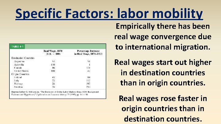
Specific Factors: labor mobility Empirically there has been real wage convergence due to international migration. Real wages start out higher in destination countries than in origin countries. Real wages rose faster in origin countries than in destination countries.