Unit 1 Measurements Uncertainties Part 2 Uncertainty Error

Unit 1: Measurements & Uncertainties Part 2 – Uncertainty & Error

Table of Contents Types of Uncertainty Calculating Uncertainty Propagated Uncertainty

Physics is an experimental science. No measurement can be infinitely accurate – there will always be some uncertainty. Types of Uncertainty: Systematic Error – Uncertainty due to an incorrectly calibrated instrument Random Error – Uncertainty due to human imperfection or difficulty reading instruments.

Systematic Uncertainty Note: Systematic Errors will always be biased in the same direction. Examples: Using a ruler on a hot day – The ruler will expand in the heat, so all measurements will be too small. Using a scale which reads 0. 5 grams even when empty – Every measurement will be too large. Doing more measurements won’t help with systematic errors.

Random Uncertainty In contrast, random errors can be biased in either direction. Examples: Timing an event with a stopwatch Estimating a length which falls between the tick marks of a ruler In the first case, random uncertainty is due to the procedure used – the accuracy of a stopwatch is limited by the reaction time of the user. In the second case, random uncertainty is due to the equipment used – the accuracy is limited by the precision of the ruler. This type of random uncertain is called a “reading uncertainty” since there is a limit to how accurately you can read the measurment.

Reading Uncertainty Note: Reading Uncertainties are always equal to half the smallest unit of precision indicated on the device used for measuring. Example: If you use a ruler with tick marks every mm, your measurements should be recorded ± 0. 5 mm or ± 0. 05 cm

Some vocab Suppose a value is recorded as a = a 0 ± Δa a 0 = the best estimate or mean value Δa = the absolute uncertainty Δa/a 0 = the fractional uncertainty (Δa/a 0) × 100% = percent uncertainty

Example Suppose a length is determined to be: L = 42. 6 cm ± 0. 1 cm The best estimate for this length is 42. 6 cm The absolute uncertainty for this length is 0. 1 cm The fraction uncertainty here = 0. 1 cm/42. 6 cm = 0. 0023 The %-uncertainty = (0. 1 cm/42. 6 cm)× 100% = 0. 23% Note: Δa and a 0 must have the same units to calculate fractional and %-uncertainty. Also note: We will use the convention that any final absolute uncertainty can have only one significant figure

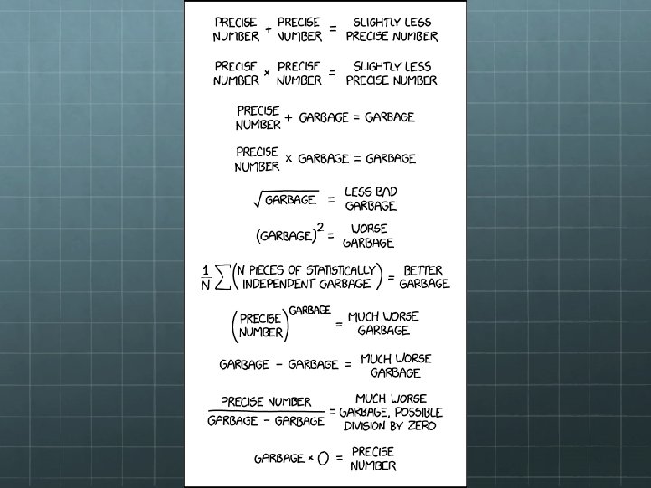
Propagation of Uncertainty If you measure a value, and then use that value to calculate something, the uncertainty in the initial value will propagate into uncertainty in the final result. How bad the final uncertainty is depends on how bad the initial uncertainties were that went into the calculation, and what type of calculation did you do. The following xkcd cartoon nicely summarizes things….

How to Calculate Propagated Uncertainty Let a, b, and c be directly measured values such that: a = a 0 + Δa b = b 0 + Δb c = c 0 + Δc If Q is a new quantity calculated from a, b, and/or c, there are two rules for how to determine uncertainty in Q: Rule #1: If Q is calculated by adding or subtracting a, b, and c, then the absolute uncertainty of Q equals the sum of the absolute uncertainties of a, b, and c: Example: If Q = a + b – c , then ΔQ = Δa + Δb + Δc

How to Calculate Propagated Uncertainty Rule #2: If Q is calculated by multiplying or dividing a, b, and c, then the fractional uncertainty of Q equals the sum of the fractional uncertainties of a, b, and c: Example: If Q = ab/c , then ΔQ = Δa + Δb + Δc Q 0 a 0 b 0 c 0 Since any expression written as an exponent can also be written as a product (for example, a 4 = a×a×a×a) one can show the following corollary to Rule #2: If Q = an, then ΔQ = |n|×Δa a 0 Q 0

Example Problem A The dimensions of a rectangle are measured to be 8. 0 cm ± 0. 1 cm and 13. 0 cm ± 0. 05 cm. Find the perimeter and area of the rectangle, including absolute error. Let’s find perimeter first: P 0 = L 0 + w 0 = 2(8. 0 cm) + 2(13. 0 cm) = 42. 0 cm Since we’re adding to get P, we use Rule #1: ΔP 0 = ΔL 0 + Δw 0 +Δ w 0 = 2(0. 1 cm) + 2(0. 05 cm) = 0. 3 cm So P = 42. 0 cm ± 0. 3 cm

Now let’s find area: A 0 = L 0 w 0 = (8. 0 cm)(13. 0 cm) = 104 cm 2 Since we’re multiplying to get A, we use Rule #2: ΔA/ = ΔL/ + Δw/ A 0 L 0 w 0 ΔA/ 0. 1 cm/ 0. 05 cm/ = + 104 cm^2 8. 0 cm 13. 0 cm Solving for ΔA yields 1. 7 cm 2. But final absolute uncertainties should have only one significant figure, so ΔA ≈ 2 cm 2 So A = 104 cm 2 ± 2 cm 2

Example Problem B A mass is measured to be 4. 4 kg ± 0. 2 kg and its speed is measured to be 18 m/s ± 2 m/s. The formula for kinetic energy is K = ½mv 2, where K = kinetic energy in joules if mass m is measured in kg and velocity v is measured in m/s. Find the kinetic energy of the mass, including absolute uncertainty. Let’s find best estimate first: K 0 = ½ m 0 v 02 = ½ (4. 4 kg)(18 m/s)2 = 712. 8 J

Since we’re multiplying to get K, we use Rule #2: ΔK/ = Δm/ Δv K 0 m 0 + 2 /v 0 (Note: the 2 is due to the exponent on the v) ΔK/ 0. 2 kg/ 2 m/s/ 712. 8 J = 4. 4 kg + 2( 18 m/s) Solving for ΔK yields 190. 8 J. But final absolute uncertainties should have only 1 sig fig. So ΔK = 200 J Since our uncertain in energy ΔK is measured in hundreds of joules, it doesn’t make sense to report our best estimate K 0 for energy to a greater level of precision that. K 0 = 712. 8 J ≈ 700 J So our final answer is: K = 700 J ± 200 J