Unit 1 Basics of Data Mining 662021 1

Unit 1: Basics of Data Mining 6/6/2021 1

6/6/2021 Data Mining: Concepts and Techniques 2

Chapter 1. Introduction Motivation: Why data mining? What is data mining? Data Mining: On what kind of data? Data mining functionality Classification of data mining systems Top-10 most popular data mining algorithms Major issues in data mining 6/6/2021 Data Mining: Concepts and Techniques 3

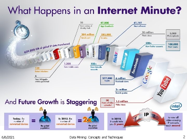
Why Data Mining? The Explosive Growth of Data: from terabytes to petabytes Ex. Wal. Mart handles 100’s of millions of transactions per week. Data collection and data availability Automated data collection tools, database systems. . Business: Web, e-commerce, transactions, stocks trading records, … Science: Remote sensing, bioinformatics… Society and everyone: news, digital cameras, You. Tube We are drowning in data, but starving for knowledge! 6/6/2021 Data Mining: Concepts and Techniques 4

“Necessity is the mother of invention”—Data mining—Automated analysis of massive data sets. Data volume too large for classical analysis Number of records too large (millions or billions) High dimensional (attributes/features/ fields) data 6/6/2021 Data Mining: Concepts and Techniques 5

Evolution of Database Technology 1960 s: Data collection, database creation, DBMS 1970 s: Relational data model, relational DBMS implementation 1980 s: RDBMS, advanced data models (extended-relational, OO, deductive, etc. ) Application-oriented DBMS (spatial, scientific, engineering, etc. ) 1990 s: Data mining, data warehousing, multimedia databases, and Web databases 2000 s Stream data management and mining Data mining and its applications Web technology (XML, data integration) and global information systems 6/6/2021 Data Mining: Concepts and Techniques 6

What Is Data Mining? Data mining (knowledge discovery from data) The iterative and interactive process of discovering valid, novel, useful, and understandable knowledge ( patterns, models, rules etc. ) in Massive databases 6/6/2021 Data Mining: Concepts and Techniques 7

What Is Data Mining? Valid: generalize to the future Novel: what we don't know Useful: be able to take some action Understandable: leading to insight Iterative: takes multiple passes Interactive: human in the loop 6/6/2021 Data Mining: Concepts and Techniques 8

What Is Data Mining? Alternative names Knowledge discovery (mining) in databases (KDD), knowledge extraction, data/pattern analysis, data archeology, data dredging, information harvesting, business intelligence, etc. 6/6/2021 Data Mining: Concepts and Techniques 9

Data mining goals Prediction What? Opaque Description Why? Transparent 6/6/2021 Data Mining: Concepts and Techniques 10

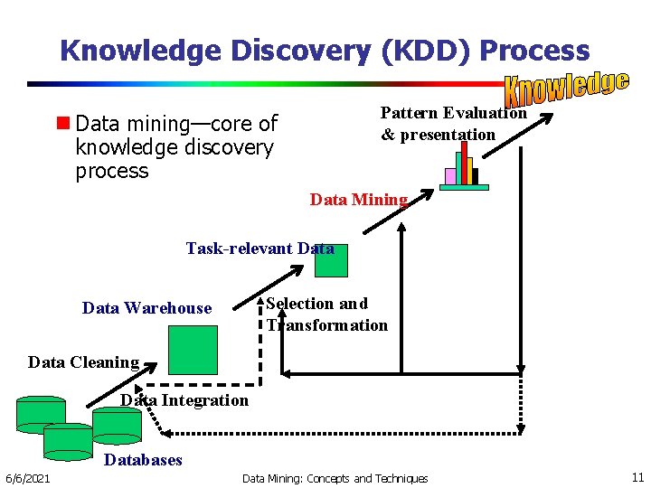
Knowledge Discovery (KDD) Process Pattern Evaluation & presentation Data mining—core of knowledge discovery process Data Mining Task-relevant Data Selection and Transformation Data Warehouse Data Cleaning Data Integration Databases 6/6/2021 Data Mining: Concepts and Techniques 11

Data mining process 1. Data Cleaning: find missing values , Remove noise(variance or random error Method: Binning), outliers, inconsistent data. 2. Data Integration: where multiple data sources may be combined. Data may be stored in data warehouse. (duplicate attribute, tuples, redundancy(derived attribute), unit of measures) 3. Data Selection: where data relevant to the analysis task are retrieved from the database. 4. Data Transformation: Where data are transformed and consolidated into forms appropriate for mining by performing summary or aggregation operations. 6/6/2021 Data Mining: Concepts and Techniques 12

5. Data Mining: Apply data mining algorithm Associations, classification, clustering, sequences etc. to extract data patterns. 6. Pattern Evaluation: To Identify the truly interesting patterns representing knowledge. 7. Knowledge Presentation: Where visualization and knowledge representation techniques are used to present mined knowledge to users. 6/6/2021 Data Mining: Concepts and Techniques 13

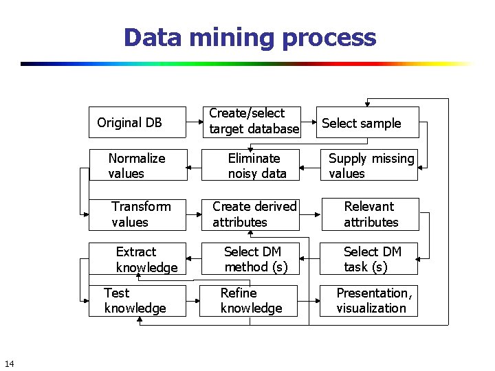
Data mining process Original DB Normalize values Transform values Extract knowledge Test knowledge 14 Create/select target database Select sample Eliminate noisy data Supply missing values Create derived attributes Relevant attributes Select DM method (s) Select DM task (s) Refine knowledge Presentation, visualization

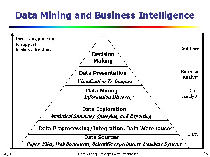
Data Mining and Business Intelligence Increasing potential to support business decisions Decision Making Data Presentation Visualization Techniques End User Business Analyst Data Mining Information Discovery Data Analyst Data Exploration Statistical Summary, Querying, and Reporting Data Preprocessing/Integration, Data Warehouses Data Sources Paper, Files, Web documents, Scientific experiments, Database Systems 6/6/2021 Data Mining: Concepts and Techniques DBA 15

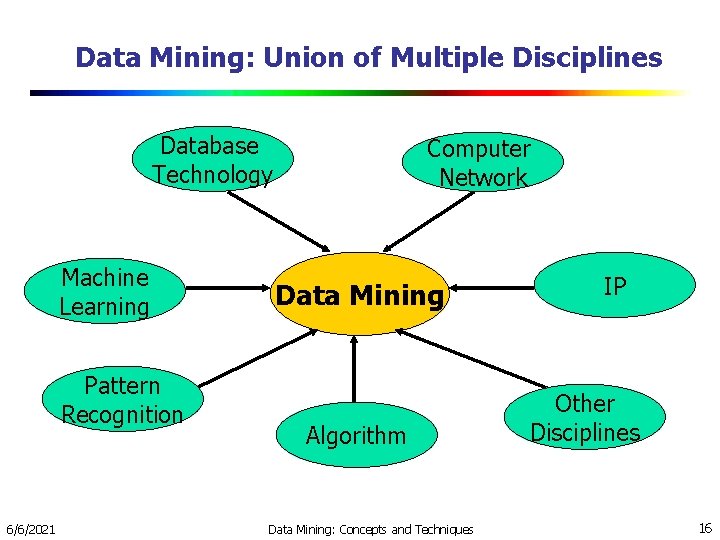
Data Mining: Union of Multiple Disciplines Database Technology Machine Learning Pattern Recognition 6/6/2021 Computer Network Data Mining Algorithm Data Mining: Concepts and Techniques IP Other Disciplines 16

Why Not Traditional Data Analysis? Tremendous amount of data Algorithms must be highly scalable to handle such as tera-bytes of data High-dimensionality of data Data may have tens of thousands of dimensions High complexity of data Data streams and sensor data Time-series data, temporal data, sequence data Structure data, graphs, social networks and multi-linked data Heterogeneous databases Spatial, multimedia, text and Web data New and sophisticated applications 6/6/2021 Data Mining: Concepts and Techniques 17

Multi-Dimensional View of Data Mining What Kinds of Data can be mined? Relational, data warehouse, transactional, stream, objectoriented/relational, spatial, time-series, text, multi-media, heterogeneous, WWW. What Kinds of pattern/Knowledge can be mined? Frequent patterns, association, Regression (predict missing or unavailable numerical values from previous data Ex. Revenue of product), classification, clustering (Maximizing intra-class similarity & minimizing interclass similarity Ex. customer location in a city), outlier analysis(Data object that does not comply with the general behavior of the data) , Characterization(summarization Ex. Features of s/w products whose sale is increased by 10% than previous year, discrimination (Ex. Customer who purchase computer regularly or rarely)etc. 6/6/2021 Data Mining: Concepts and Techniques 18

Techniques utilized Database-oriented, data warehouse (OLAP), machine learning, statistics, visualization, etc. Applications adapted Retail, telecommunication, banking, fraud analysis, Business Intelligence, stock market analysis, text mining, Web search engines(D. M. is used in phases like crawling , indexing, ranking) etc. 6/6/2021 Data Mining: Concepts and Techniques 19

Top-10 Algorithm #1: C 4. 5 (61 votes) #2: K-Means (60 votes) #3: SVM (58 votes) #4: Apriori (52 votes) #5: EM (Expectation Maximization) (48 votes) #6: Page. Rank (46 votes) #7: Ada. Boost (45 votes) #7: k. NN (45 votes) #7: Naive Bayes (45 votes) #10: CART(classification and regression tree) (34 votes) 6/6/2021 Data Mining: Concepts and Techniques 20

Major Issues in Data Mining methodology Mining different kinds of knowledge from diverse data types, e. g. , bio, stream, Web, temporal data, spatial data. (It is unrealistic to expect one data mining system to mine all kinds of data. ) Performance: efficiency, effectiveness, and scalability(D. M. algorithm should be efficient and scalable to extract from huge amount of data in data repository) Pattern evaluation: the interestingness problem(all patterns are not interesting) Incorporation of background knowledge(constraints, rules, information of domain need to be incorporated in process. ) Handling noise and incomplete data Integration of the discovered knowledge with existing one: knowledge fusion 6/6/2021 Data Mining: Concepts and Techniques 21

User interaction Data mining query languages and ad-hoc mining Presentation and visualization of data mining results. (knowledge should be understandable and usable. ) Interactive mining(how to interact with the data mining system. ): It allows to change the focus of a search and refine the results Ex. Drill, dice etc. Data mining and society: Domain-specific data mining & invisible data mining: we can’t expect everyone is knowing about D. M. techniques in the society. So try to incorporate it in the components. So that with mouse click user may use the data mining technique without prior knowledge. Ex. Purchasing items online(from our buying patterns we may get recommendation for other items in future. ) 6/6/2021 Data Mining: Concepts and Techniques 22

Protection of data security, integrity, and privacy(ex. Real time discovery of intruders and cyber attacks. ) Need to observe data sensitivity and preserve peoples privacy while performing successful data mining. 6/6/2021 Data Mining: Concepts and Techniques 23

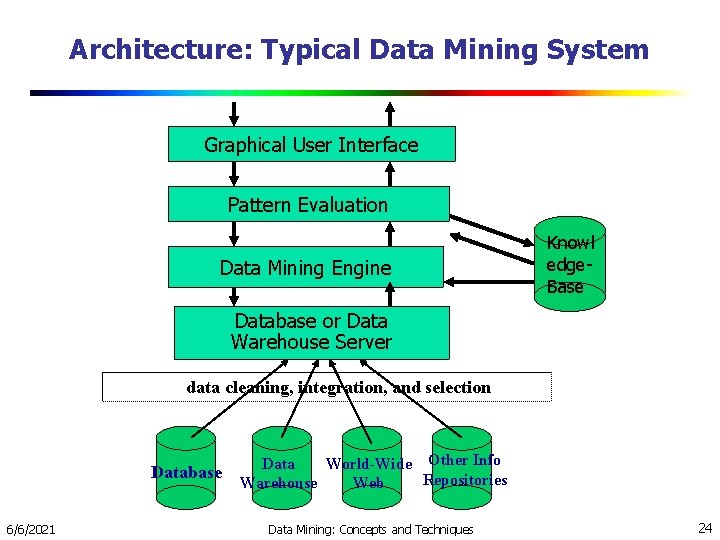
Architecture: Typical Data Mining System Graphical User Interface Pattern Evaluation Data Mining Engine Knowl edge. Base Database or Data Warehouse Server data cleaning, integration, and selection Database 6/6/2021 Data World-Wide Other Info Repositories Warehouse Web Data Mining: Concepts and Techniques 24

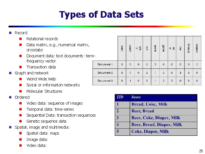
Types of Data Sets Record Relational records Data matrix, e. g. , numerical matrix, crosstabs Document data: text documents: termfrequency vector Transaction data Graph and network World Wide Web Social or information networks Molecular Structures Ordered Video data: sequence of images Temporal data: time-series Sequential Data: transaction sequences Genetic sequence data Spatial, image and multimedia: Spatial data: maps Image data: Video data: 25

Important Characteristics of Structured Data Dimensionality Curse of dimensionality Sparsity Only presence counts Resolution Patterns depend on the scale Distribution Centrality and dispersion 26

Data Objects Data sets are made up of data objects. A data object represents an entity. Examples: sales database: customers, store items, sales medical database: patients, treatments university database: students, professors, courses Also called samples , examples, instances, data points, objects, tuples. Data objects are described by attributes. Database rows -> data objects; columns ->attributes. 27

Attributes Attribute (or dimensions, features, variables): a data field, representing a characteristic or feature of a data object. E. g. , customer _ID, name, address Types: Nominal Binary Numeric: quantitative Interval-scaled Ratio-scaled 28

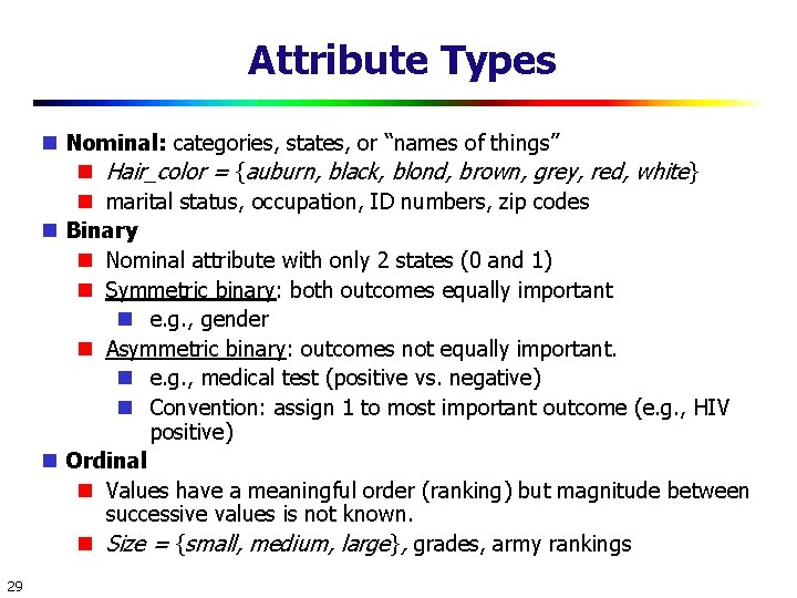
Attribute Types Nominal: categories, states, or “names of things” Hair_color = {auburn, black, blond, brown, grey, red, white} marital status, occupation, ID numbers, zip codes Binary Nominal attribute with only 2 states (0 and 1) Symmetric binary: both outcomes equally important e. g. , gender Asymmetric binary: outcomes not equally important. e. g. , medical test (positive vs. negative) Convention: assign 1 to most important outcome (e. g. , HIV positive) Ordinal Values have a meaningful order (ranking) but magnitude between successive values is not known. Size = {small, medium, large}, grades, army rankings 29

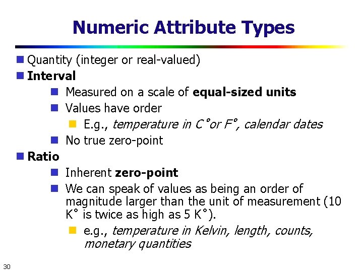
Numeric Attribute Types Quantity (integer or real-valued) Interval Measured on a scale of equal-sized units Values have order E. g. , temperature in C˚or F˚, calendar dates No true zero-point Ratio Inherent zero-point We can speak of values as being an order of magnitude larger than the unit of measurement (10 K˚ is twice as high as 5 K˚). e. g. , temperature in Kelvin, length, counts, monetary quantities 30

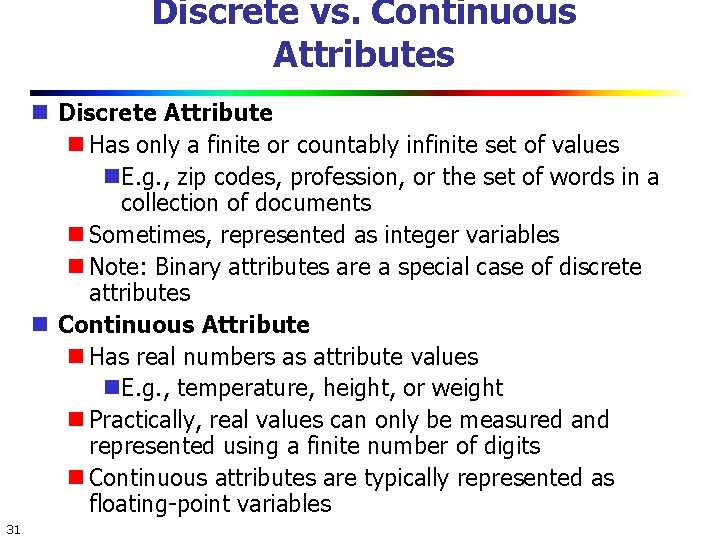
Discrete vs. Continuous Attributes Discrete Attribute Has only a finite or countably infinite set of values E. g. , zip codes, profession, or the set of words in a collection of documents Sometimes, represented as integer variables Note: Binary attributes are a special case of discrete attributes Continuous Attribute Has real numbers as attribute values E. g. , temperature, height, or weight Practically, real values can only be measured and represented using a finite number of digits Continuous attributes are typically represented as floating-point variables 31

Chapter 3: Data Preprocessing: An Overview Data Quality Major Tasks in Data Preprocessing Data Cleaning Data Integration Data Reduction Data Transformation and Data Discretization Summary 32

Data Quality: Why Preprocess the Data? Measures for data quality: A multidimensional view Accuracy: correct or wrong, accurate or not Completeness: not recorded, unavailable, … Consistency: some modified but some not, dangling, … Timeliness: timely update? Believability: how trustable the data are correct? Interpretability: how easily the data can be understood? 33

Major Tasks in Data Preprocessing Data cleaning Fill in missing values, smooth noisy data, identify or remove outliers, and resolve inconsistencies Data integration Integration of multiple databases, data cubes, or files Data reduction Dimensionality reduction Numerosity reduction Data compression Data transformation and data discretization Normalization Concept hierarchy generation 34

Chapter 3: Data Preprocessing: An Overview Data Quality Major Tasks in Data Preprocessing Data Cleaning Data Integration Data Reduction Data Transformation and Data Discretization Summary 35

Data Cleaning Data in the Real World Is Dirty: Lots of potentially incorrect data, e. g. , instrument faulty, human or computer error, transmission error incomplete: lacking attribute values, lacking certain attributes of interest, or containing only aggregate data e. g. , Occupation=“ ” (missing data) noisy: containing noise, errors, or outliers e. g. , Salary=“− 10” (an error) inconsistent: containing discrepancies in codes or names, e. g. , Age=“ 42”, Birthday=“ 03/07/2010” Was rating “ 1, 2, 3”, now rating “A, B, C” discrepancy between duplicate records Intentional (e. g. , disguised missing data) Jan. 1 as everyone’s birthday? 36

Incomplete (Missing) Data is not always available E. g. , many tuples have no recorded value for several attributes, such as customer income in sales data Missing data may be due to equipment malfunction inconsistent with other recorded data and thus deleted data not entered due to misunderstanding certain data may not be considered important at the time of entry not register history or changes of the data Missing data may need to be inferred 37

How to Handle Missing Data? Ignore the tuple: usually done when class label is missing (when doing classification)—not effective when the % of missing values per attribute varies considerably Fill in the missing value manually: tedious + infeasible? Fill in it automatically with a global constant : e. g. , “unknown”, a new class? ! the attribute mean for all samples belonging to the same class: smarter the most probable value: inference-based such as Bayesian formula or decision tree 38

Noisy Data Noise: random error or variance in a measured variable Incorrect attribute values may be due to faulty data collection instruments data entry problems data transmission problems technology limitation inconsistency in naming convention Other data problems which require data cleaning duplicate records incomplete data inconsistent data 39

How to Handle Noisy Data? Binning first sort data and partition into (equal-frequency) bins then one can smooth by bin means, smooth by bin median, smooth by bin boundaries, etc. Regression smooth by fitting the data into regression functions Clustering detect and remove outliers Combined computer and human inspection detect suspicious values and check by human (e. g. , deal with possible outliers) 40

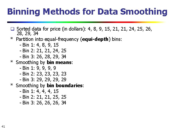
Binning Methods for Data Smoothing Sorted data for price (in dollars): 4, 8, 9, 15, 21, 24, 25, 26, 28, 29, 34 * Partition into equal-frequency (equi-depth) bins: - Bin 1: 4, 8, 9, 15 - Bin 2: 21, 24, 25 - Bin 3: 26, 28, 29, 34 * Smoothing by bin means: - Bin 1: 9, 9, 9, 9 - Bin 2: 23, 23, 23 - Bin 3: 29, 29, 29 * Smoothing by bin boundaries: - Bin 1: 4, 4, 4, 15 - Bin 2: 21, 25, 25 - Bin 3: 26, 26, 34 41

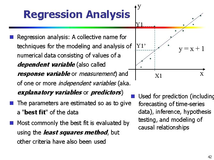
Regression Analysis y Y 1 Regression analysis: A collective name for techniques for the modeling and analysis of Y 1’ numerical data consisting of values of a y=x+1 dependent variable (also called x response variable or measurement) and X 1 of one or more independent variables (aka. explanatory variables or predictors) Used for prediction (including The parameters are estimated so as to give a "best fit" of the data Most commonly the best fit is evaluated by using the least squares method, but forecasting of time-series data), inference, hypothesis testing, and modeling of causal relationships other criteria have also been used 42

Histogram Analysis Divide data into buckets and store average (sum) for each bucket Partitioning rules: Equal-width: equal bucket range Equal-frequency (or equaldepth) 44

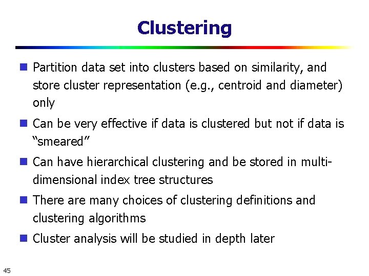
Clustering Partition data set into clusters based on similarity, and store cluster representation (e. g. , centroid and diameter) only Can be very effective if data is clustered but not if data is “smeared” Can have hierarchical clustering and be stored in multidimensional index tree structures There are many choices of clustering definitions and clustering algorithms Cluster analysis will be studied in depth later 45

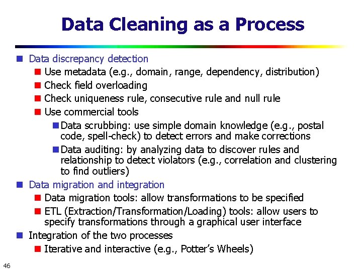
Data Cleaning as a Process Data discrepancy detection Use metadata (e. g. , domain, range, dependency, distribution) Check field overloading Check uniqueness rule, consecutive rule and null rule Use commercial tools Data scrubbing: use simple domain knowledge (e. g. , postal code, spell-check) to detect errors and make corrections Data auditing: by analyzing data to discover rules and relationship to detect violators (e. g. , correlation and clustering to find outliers) Data migration and integration Data migration tools: allow transformations to be specified ETL (Extraction/Transformation/Loading) tools: allow users to specify transformations through a graphical user interface Integration of the two processes Iterative and interactive (e. g. , Potter’s Wheels) 46

Chapter 3: Data Preprocessing: An Overview Data Quality Major Tasks in Data Preprocessing Data Cleaning Data Integration Data Reduction Data Transformation and Data Discretization Summary 47

Data Integration Data integration: Combines data from multiple sources into a coherent store Schema integration: e. g. , A. cust-id B. cust-# Integrate metadata from different sources Entity identification problem: Identify real world entities from multiple data sources, e. g. , Bill Clinton = William Clinton Detecting and resolving data value conflicts For the same real world entity, attribute values from different sources are different Possible reasons: different representations, different scales, e. g. , metric vs. British units 48 48

Handling Redundancy in Data Integration Redundant data occur often when integration of multiple databases Object identification: The same attribute or object may have different names in different databases Derivable data: One attribute may be a “derived” attribute in another table, e. g. , annual revenue Redundant attributes may be able to be detected by correlation analysis and covariance analysis Careful integration of the data from multiple sources may help reduce/avoid redundancies and inconsistencies and improve mining speed and quality 49 49

Data Reduction Strategies Data reduction: Obtain a reduced representation of the data set that is much smaller in volume but yet produces the same (or almost the same) analytical results Why data reduction? — A database/data warehouse may store terabytes of data. Complex data analysis may take a very long time to run on the complete data set. Data reduction strategies Dimensionality reduction, e. g. , remove unimportant attributes Wavelet transforms Principal Components Analysis (PCA) Feature subset selection, feature creation Numerosity reduction (some simply call it: Data Reduction) Regression and Log-Linear Models Histograms, clustering, sampling Data cube aggregation Data compression 50

Data Reduction 1: Dimensionality Reduction Curse of dimensionality When dimensionality increases, data becomes increasingly sparse Density and distance between points, which is critical to clustering, outlier analysis, becomes less meaningful The possible combinations of subspaces will grow exponentially Dimensionality reduction Avoid the curse of dimensionality Help eliminate irrelevant features and reduce noise Reduce time and space required in data mining Allow easier visualization Dimensionality reduction techniques Wavelet transforms Principal Component Analysis Supervised and nonlinear techniques (e. g. , feature selection) 51

Data Cube Aggregation The lowest level of a data cube (base cuboid) The aggregated data for an individual entity of interest E. g. , a customer in a phone calling data warehouse Multiple levels of aggregation in data cubes Further reduce the size of data to deal with Reference appropriate levels Use the smallest representation which is enough to solve the task Queries regarding aggregated information should be answered using data cube, when possible 52

Data Transformation A function that maps the entire set of values of a given attribute to a new set of replacement values s. t. each old value can be identified with one of the new values Methods Smoothing: Remove noise from data Attribute/feature construction New attributes constructed from the given ones Aggregation: Summarization, data cube construction Normalization: Scaled to fall within a smaller, specified range min-max normalization z-score normalization by decimal scaling Discretization: Concept hierarchy climbing 53

Normalization Min-max normalization: to [new_min. A, new_max. A] Ex. Let income range $12, 000 to $98, 000 normalized to [0. 0, 1. 0]. Then $73, 000 is mapped to Z-score normalization (μ: mean, σ: standard deviation): Ex. Let μ = 54, 000, σ = 16, 000. Then Decimal Scaling: Suppose values are in range -986 to 917, the maximum absolute value is 986 hence devide each value by 1000 so -986 becomes -0. 986 And 917 becomes 0. 917 54

Discretization Three types of attributes Nominal—values from an unordered set, e. g. , color, profession Ordinal—values from an ordered set, e. g. , military or academic rank Numeric—real numbers, e. g. , integer or real numbers Discretization: Divide the range of a continuous attribute into intervals Interval labels can then be used to replace actual data values Reduce data size by discretization Supervised vs. unsupervised Split (top-down) vs. merge (bottom-up) Discretization can be performed recursively on an attribute Prepare for further analysis, e. g. , classification 55

Data Discretization Methods Typical methods: All the methods can be applied recursively Binning Top-down split, unsupervised Histogram analysis Top-down split, unsupervised Clustering analysis (unsupervised, top-down split or bottom-up merge) Decision-tree analysis (supervised, top-down split) Correlation (e. g. , 2) analysis (unsupervised, bottom-up merge) 56

Simple Discretization: Binning Equal-width (distance) partitioning Divides the range into N intervals of equal size: uniform grid if A and B are the lowest and highest values of the attribute, the width of intervals will be: W = (B –A)/N. The most straightforward, but outliers may dominate presentation Skewed data is not handled well Equal-depth (frequency) partitioning Divides the range into N intervals, each containing approximately same number of samples Good data scaling Managing categorical attributes can be tricky 57

Discretization by Classification & Correlation Analysis Classification (e. g. , decision tree analysis) Supervised: Given class labels, e. g. , cancerous vs. benign Using entropy to determine split point (discretization point) Top-down, recursive split Details to be covered in Chapter 7 Correlation analysis (e. g. , Chi-merge: χ2 -based discretization) Supervised: use class information Bottom-up merge: find the best neighboring intervals (those having similar distributions of classes, i. e. , low χ2 values) to merge Merge performed recursively, until a predefined stopping condition 58

Concept Hierarchy Generation Concept hierarchy organizes concepts (i. e. , attribute values) hierarchically and is usually associated with each dimension in a data warehouse Concept hierarchies facilitate drilling and rolling in data warehouses to view data in multiple granularity Concept hierarchy formation: Recursively reduce the data by collecting and replacing low level concepts (such as numeric values for age) by higher level concepts (such as youth, adult, or senior) Concept hierarchies can be explicitly specified by domain experts and/or data warehouse designers Concept hierarchy can be automatically formed for both numeric and nominal data. For numeric data, use discretization methods shown. 59

Concept Hierarchy Generation for Nominal Data Specification of a partial/total ordering of attributes explicitly at the schema level by users or experts street < city < state < country Specification of a hierarchy for a set of values by explicit data grouping {Urbana, Champaign, Chicago} < Illinois Specification of only a partial set of attributes E. g. , only street < city, not others Automatic generation of hierarchies (or attribute levels) by the analysis of the number of distinct values E. g. , for a set of attributes: {street, city, state, country} 60

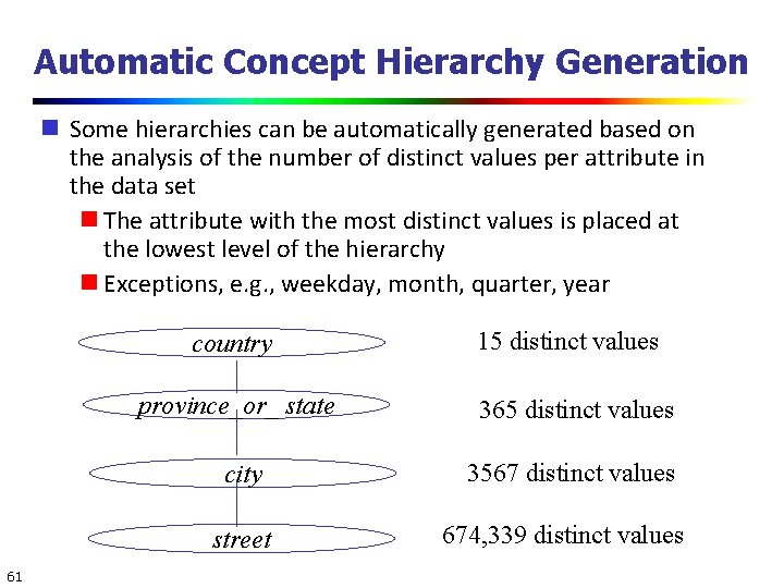
Automatic Concept Hierarchy Generation Some hierarchies can be automatically generated based on the analysis of the number of distinct values per attribute in the data set The attribute with the most distinct values is placed at the lowest level of the hierarchy Exceptions, e. g. , weekday, month, quarter, year country province_or_ state 365 distinct values city 3567 distinct values street 61 15 distinct values 674, 339 distinct values

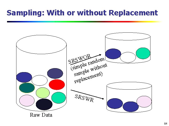
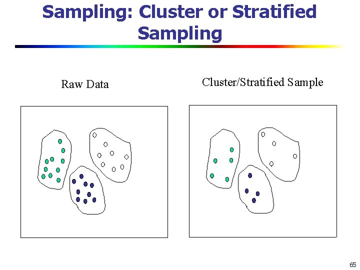
Sampling Sampling: obtaining a small sample s to represent the whole data set N Allow a mining algorithm to run in complexity that is potentially sub-linear to the size of the data Key principle: Choose a representative subset of the data Simple random sampling may have very poor performance in the presence of skew Develop adaptive sampling methods, e. g. , stratified sampling: Note: Sampling may not reduce database I/Os (page at a time) 62

Types of Sampling Simple random sampling There is an equal probability of selecting any particular item Sampling without replacement Once an object is selected, it is removed from the population Sampling with replacement A selected object is not removed from the population Stratified sampling: Partition the data set, and draw samples from each partition (proportionally, i. e. , approximately the same percentage of the data) Used in conjunction with skewed data 63

Sampling: With or without Replacement R O W SRS le random t p u o m i h t s i ( w e l samp ment) e c a l p re SRSW R Raw Data 64

Sampling: Cluster or Stratified Sampling Raw Data Cluster/Stratified Sample 65

Data Cube Aggregation The lowest level of a data cube (base cuboid) The aggregated data for an individual entity of interest E. g. , a customer in a phone calling data warehouse Multiple levels of aggregation in data cubes Further reduce the size of data to deal with Reference appropriate levels Use the smallest representation which is enough to solve the task Queries regarding aggregated information should be answered using data cube, when possible 66

Data Reduction 3: Data Compression String compression There are extensive theories and well-tuned algorithms Typically lossless, but only limited manipulation is possible without expansion Audio/video compression Typically lossy compression, with progressive refinement Sometimes small fragments of signal can be reconstructed without reconstructing the whole Time sequence is not audio Typically short and vary slowly with time Dimensionality and numerosity reduction may also be considered as forms of data compression 67

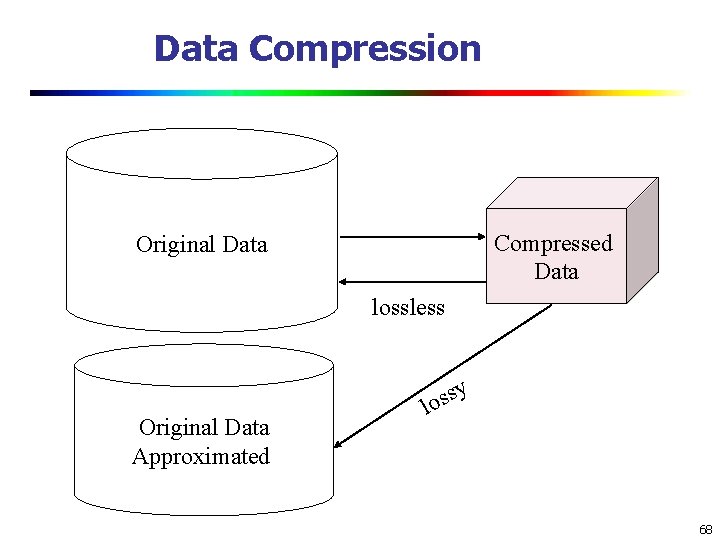
Data Compression Compressed Data Original Data lossless y Original Data Approximated s los 68