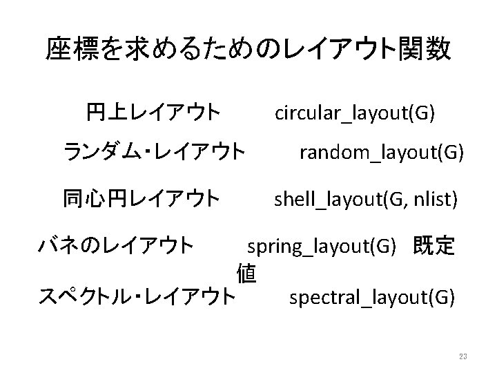
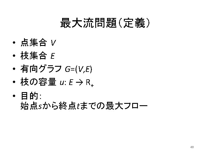
undirected graph graph GV E V node vertex


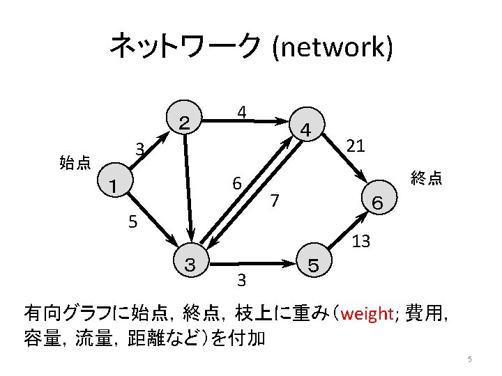
 G=(V, E) 2 4 1 6 3 5 V: 点(node, vertex,")
 Network. Xのモジュールをすべて読み込む from networkx import * G = Multi. Graph() Multi. Graph(")
![点の追加 G. add_node(1) G. add_node('Tokyo') 属性付きで追加 G. add_node(5, demand=500) G. add_node(6, product=['A', 'F', 'D'])](https://slidetodoc.com/presentation_image_h/b79ba432c0de4de3c4313ef7c43f4f83/image-10.jpg "点の追加 G. add_node(1) G. add_node('Tokyo') 属性付きで追加 G. add_node(5, demand=500) G. add_node(6, product=['A', 'F', 'D'])")
 枝の追加(点は自動的に追加される) G. add_edge(1, 2) G. add_edge(1, 3) 属性付きで追加 G. add_edge(2, 3, weight=7,")
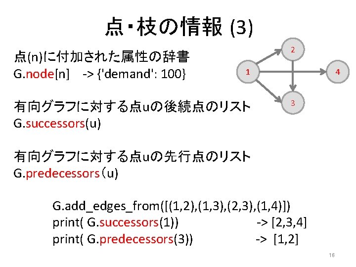
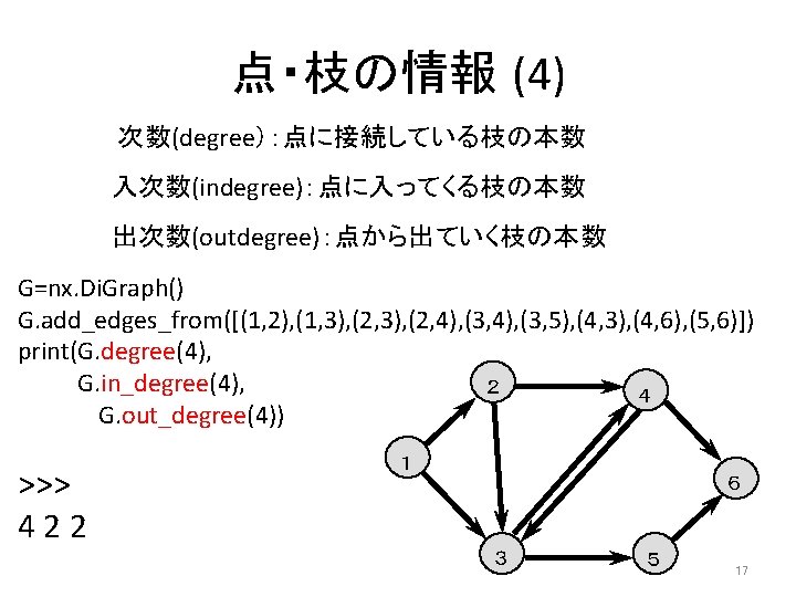
 すべての点のリスト G. nodes( ) for n in G で反復 すべての枝のリスト G. edges(")
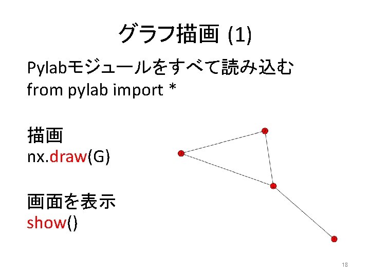
 Matplotlibのpyplotをpltという名前で読み込む import matplotlib. pyplot as plt nx. draw(G) 画面を表示 plt. show() ファイルに保存(規定値はPNGフォーマット)")
 20")
![一部の点,枝を描画 nx. draw(G, nodelist=[1, 2], edgelist=[(1, 2)]) 22](https://slidetodoc.com/presentation_image_h/b79ba432c0de4de3c4313ef7c43f4f83/image-22.jpg "一部の点,枝を描画 nx. draw(G, nodelist=[1, 2], edgelist=[(1, 2)]) 22")
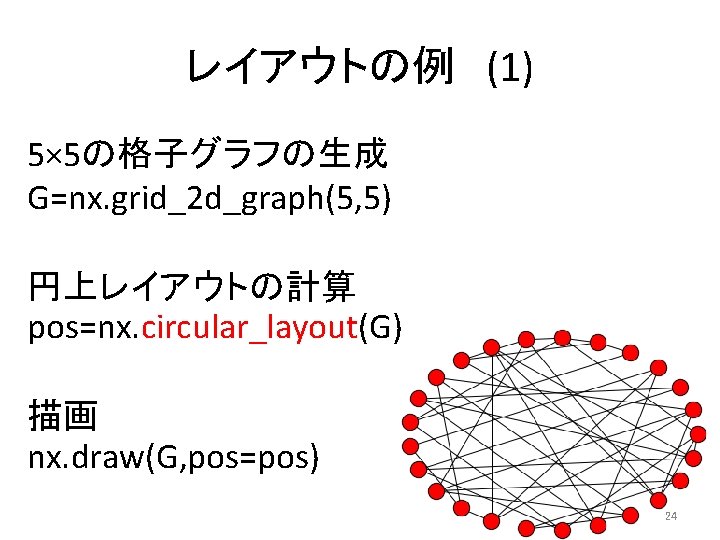
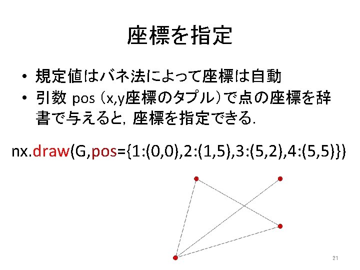
 10× 30のランダムな 2部グラフの生成 G=nx. bipartite_random_graph(10, 30, 0. 3) 同心円レイアウト(最初の 10点が内側) pos=nx. shell_layout( G,")
 c =nx. connected_components(G) -> 連結成分(点リスト)のジェネレータ nx.")
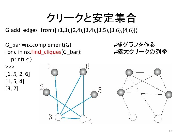
, (1, 5), (2, 3), (2, 6), (3, 4),")
 print( nx. maximal_matching(G) ) print( nx. max_weight_matching(G) ) 極大(maximal)マッチング")
 G. add_edge ('Arigator', 'Bull', weight=")
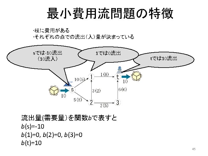
 G. add_node(‘s’, demand = -10) # 負の流出量 = 供給量 G. add_node(‘t’, demand")
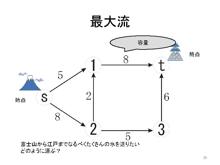
 ネットワーク単体法 network_simplex(G, demand, capacity, weight) 容量スケーリング法 capacity_scaling(G, demand, capacity, weight) 最大流+最小費用 max_flow_min_cost(G,")
 深さ優先探索(depth first search) (枝を返す場合): for e in nx. dfs_edges(G, 1): print(e) >>>")

- Slides: 60
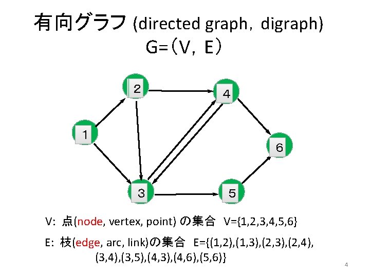
無向グラフ(undirected graph, graph) G=(V, E) 2 4 1 6 3 5 V: 点(node, vertex, point)の集合 V={1, 2, 3, 4, 5, 6} E: 枝(edge, arc, link)の集合 E={(1, 2), (1, 3), (2, 4), (3, 5), (4, 6), (5, 6)} 3
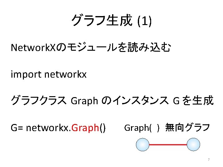
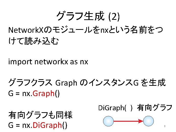
グラフ生成 (3) Network. Xのモジュールをすべて読み込む from networkx import * G = Multi. Graph() Multi. Graph( ) 多重無向グラフ G = Multi. Di. Graph() Multi. Di. Graph( ) 多重有向グラフ 9
点の追加 G. add_node(1) G. add_node('Tokyo') 属性付きで追加 G. add_node(5, demand=500) G. add_node(6, product=['A', 'F', 'D']) まとめて追加も可能 G. add_nodes_from( [ 1, 2, 3, 4 ] ) 10
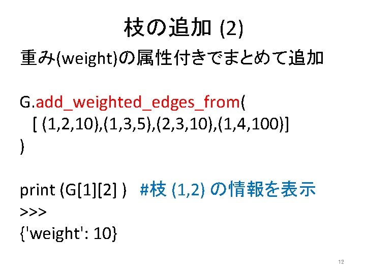
枝の追加 (1) 枝の追加(点は自動的に追加される) G. add_edge(1, 2) G. add_edge(1, 3) 属性付きで追加 G. add_edge(2, 3, weight=7, capacity=15. 0) G. add_edge(1, 4, cost=1000) まとめて追加も可能 G. add_edges_from([ (1, 2), (1, 3), (2, 3), (1, 4)]) 11
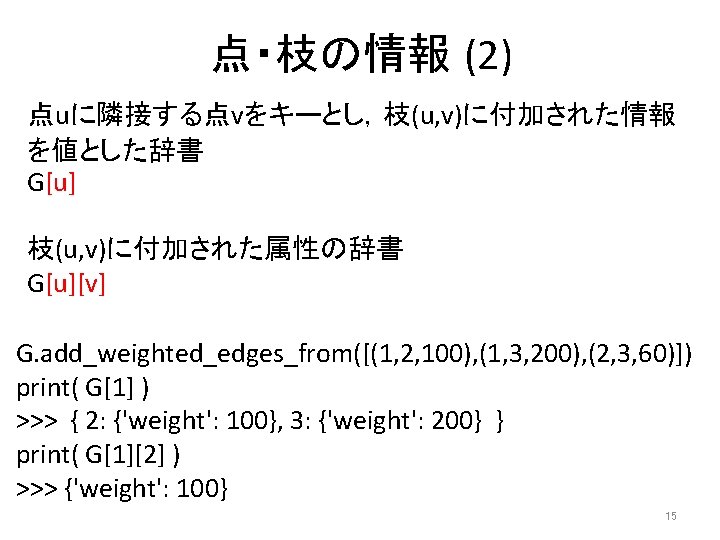
点・枝の情報 (1) すべての点のリスト G. nodes( ) for n in G で反復 すべての枝のリスト G. edges( ) for e in G. edges_iter() で反復 隣接点のリスト G. neighbors( u ) G. add_edges_from([(1, 2), (1, 3)]) for n in G: print( n, G. neighbors(n) ) 2 >>> 1 [2, 3] 1 2 [1] 3 3 [1] 14
グラフ描画 (2) Matplotlibのpyplotをpltという名前で読み込む import matplotlib. pyplot as plt nx. draw(G) 画面を表示 plt. show() ファイルに保存(規定値はPNGフォーマット) plt. savefig('sample') 19
ラベル,点の色・大きさ,枝の色・太さ を変える nx. draw(with_labels=True, G, node_color=‘r’, node_size=1000, edge_color='g', width=10) 20
一部の点,枝を描画 nx. draw(G, nodelist=[1, 2], edgelist=[(1, 2)]) 22
レイアウトの例 (2) 10× 30のランダムな 2部グラフの生成 G=nx. bipartite_random_graph(10, 30, 0. 3) 同心円レイアウト(最初の 10点が内側) pos=nx. shell_layout( G, nlist=[ [i for i in range(10)], [i for i in range(10, 40)] ] ) 描画 nx. draw(G, pos=pos) 25
連結性 連結:任意の 2点間にパスが存在 ランダムで疎な幾何学的グラフの生成 G=nx. random_geometric_graph(100, 0. 1) c =nx. connected_components(G) -> 連結成分(点リスト)のジェネレータ nx. draw(G, nodelist=list(c)[0]) nx. draw(G, nodelist=list(c)[1]) 28
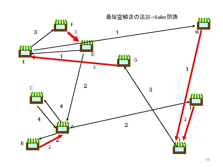
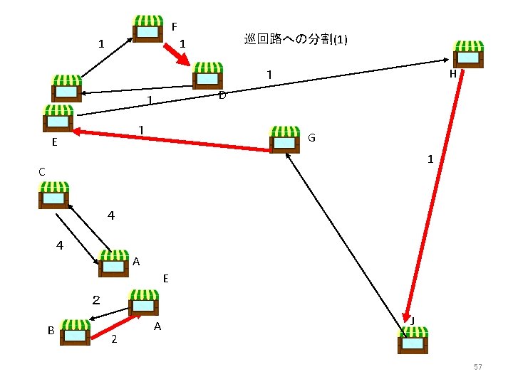
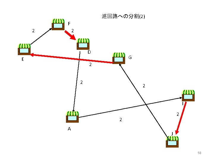
Euler閉路:すべての枝をちょうど 1回ずつ通過する閉路 G. add_edges_from([ (1, 2), (1, 5), (2, 3), (2, 6), (3, 4), (3, 7), (4, 8), (5, 6), (6, 7), (7, 8), (2, 9), (6, 9), (3, 10), (7, 10)]) print( nx. is_eulerian(G) ) >>> True for e in nx. eulerian_circuit(G): print( e , end='') >>> (1, 2) (2, 3) (3, 4) (4, 8) (8, 7) (7, 3) (3, 10) (10, 7) (7, 6) (6, 2) (2, 9) (9, 6) (6, 5) (5, 1) 33
マッチング:点の次数が1以下の部分グラフ G=nx. grid_2 d_graph(3, 4) print( nx. maximal_matching(G) ) print( nx. max_weight_matching(G) ) 極大(maximal)マッチング 最大(maximum)マッチング 34
最小木 G. add_edge ('Arigator', 'White. Bear', weight= 2 ) G. add_edge ('Arigator', 'Bull', weight= 1 ) G. add_edge ('Bull', 'White. Bear', weight= 1 ) G. add_edge ('Bull', 'Shark', weight= 3 ) G. add_edge ('White. Bear', 'Condor', weight= 3 ) G. add_edge ('White. Bear', 'Shark', weight= 5 ) G. add_edge ('Shark', 'Condor', weight= 4 ) T= nx. minimum_spanning_tree(G) Print( T. edges() ) >>> 結果 [('White. Bear', 'Condor'), ('White. Bear', 'Bull'), ('Arigator', 'Bull'), ('Shark', 'Bull')] 35
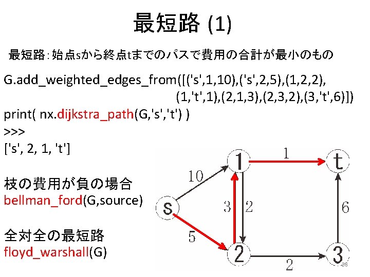
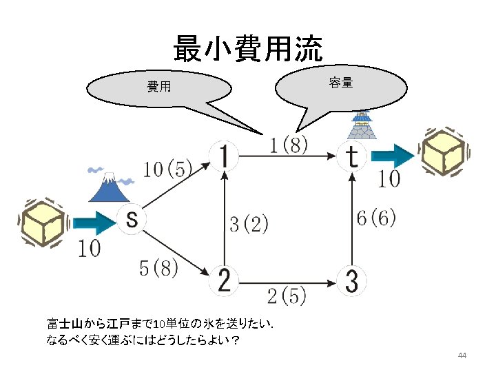
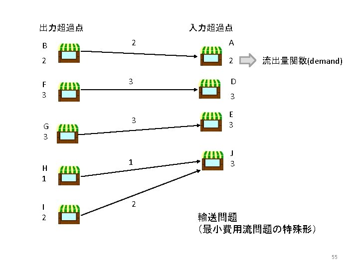
最小費用流 (1) G. add_node(‘s’, demand = -10) # 負の流出量 = 供給量 G. add_node(‘t’, demand = 10) # 正の流出量 = 需要量 G. add_edge('s', 1, weight = 10, capacity = 5) G. add_edge('s', 2, weight = 5, capacity = 8) G. add_edge(2, 1, weight = 3, capacity = 2) G. add_edge(1, 't', weight = 1, capacity = 8) G. add_edge(2, 3, weight = 2, capacity = 5) G. add_edge(3, 't', weight = 6, capacity = 6) 7 print( nx. network_simplex(G) ) >>> ((112, {1: {'t': 7}, 's': {1: 5, 2: 5}, 3: {'t': 3}, 2: {1: 2, 3: 3}, 't': {}}) 5 5 2 3 48
最小費用流 (2) ネットワーク単体法 network_simplex(G, demand, capacity, weight) 容量スケーリング法 capacity_scaling(G, demand, capacity, weight) 最大流+最小費用 max_flow_min_cost(G, s, t, capacity, weight) 49
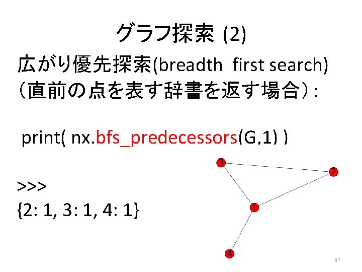
グラフ探索 (1) 深さ優先探索(depth first search) (枝を返す場合): for e in nx. dfs_edges(G, 1): print(e) >>> (1, 2) (2, 3) (1, 4) 50
Questions, Comments, Suggestions? 60