Understanding Multispectral Reflectance Remote sensing measures reflected light

Understanding Multispectral Reflectance � Remote sensing measures reflected “light” (EMR) � Different materials reflect EMR differently � Basis for distinguishing materials

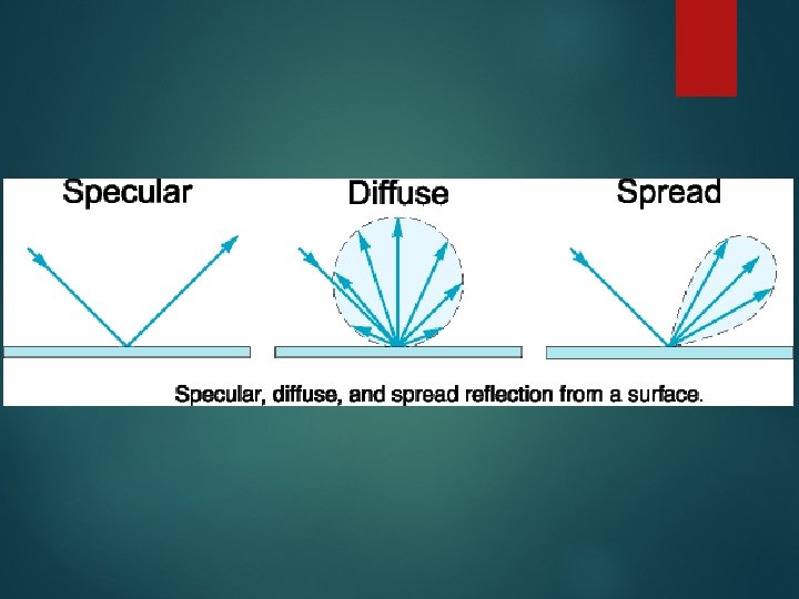
Types of Reflectance � � Specular � Mirrors or surfaces of lakes, for example � Angle of incidence = angle of reflection Diffuse (aka Lambertian) � Reflects equally in all directions � Usually we assume Lambertian reflectance for natural surfaces � Idealized—not really found in nature but often close

Reflectance of Materials � Varies with wavelength � Varies with geometry � Diagnostic of different materials What kinds of reflectance do you see here? Why do the different ponchos look different (e. g. pink vs. green)?

Some Important Terms � Irradiance (Eλ) (Incoming light from sun) � Radiance (L λ ) (Light received at satellite) Lλ Eλ

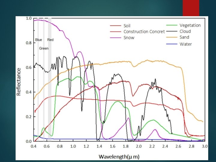
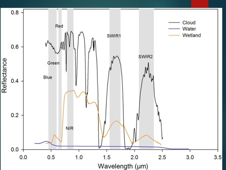
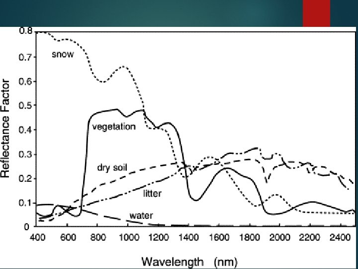
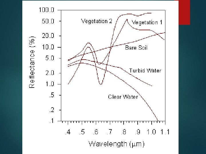
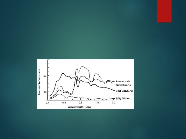
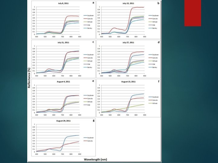
Reflectance spectra

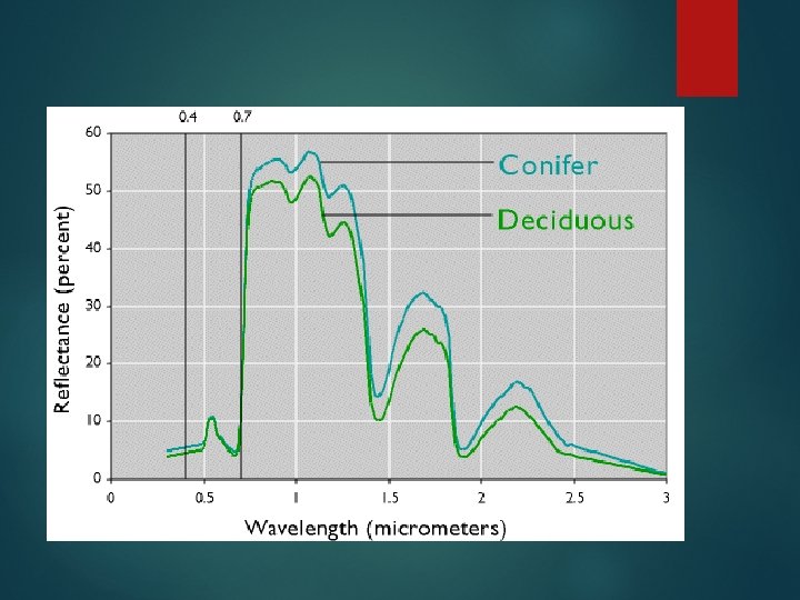
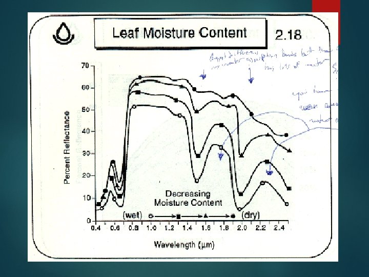
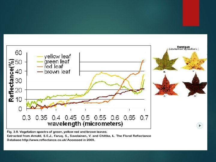
OK. What are my main variables - plants � Time of year (color) � Species (grasses, shrubs, deciduous trees, conifers. � Moisture content � Canopy layers/thickness of veg.

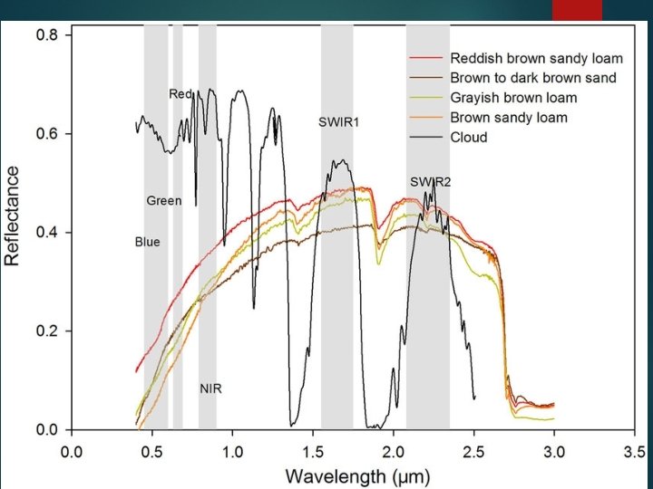
Main variables - soils � Iron � Organic content � water

Main variables – snow/ice � Age � Dust cover

Main variables - water � Turbidity � Vegetation � Scatter from waves

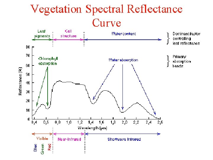
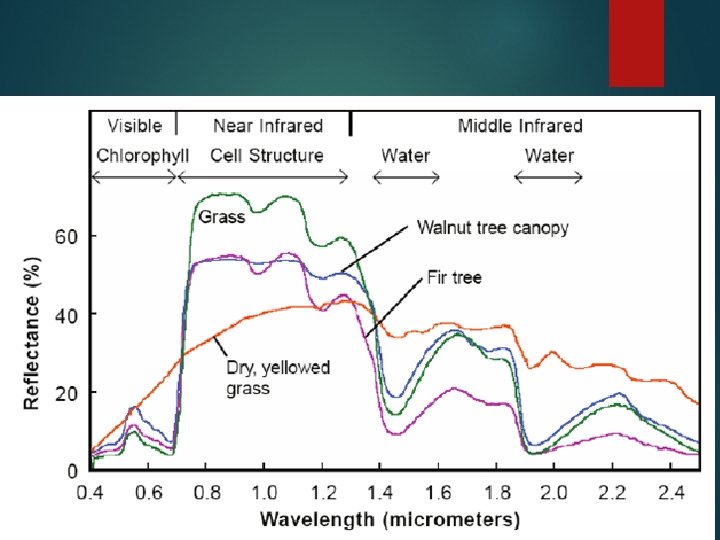
Spectral Properties of Vegetation � Unlike minerals, vegetation is composed of a limited set of spectrally active compounds � Relative abundance of compounds, including water, indicates veg. condition � Vegetation structure has significant influence on reflectance. � Spatial scale of reflectance measurement is critical.

Plant Pigments � Chlorophyll A (green) � Chlorophyll B (green) � Others: e. g. , β – carotene (yellow) and Xanthophylls (red)

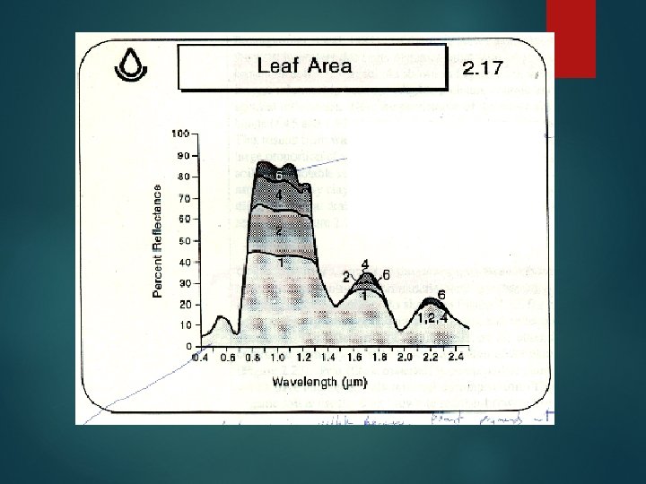
The Red Edge

Multiple Leaf Layers � Reflectance increases with the number of leaf layers in a non-linear fashion � Eventually, with enough layers, the reflectance “saturates” (stops increasing)

How do you get spectra? � Measure in the field with field spectroradiometers � Measure in the lab � Collect from image data � Look at spectral libraries: http: //speclab. cr. usgs. gov/spectral-lib. html)

Spectral Investigations

Remotely Sensed Data � Represent the amount of light reflecting off the ground and reaching the satellite sensor. � Continuous change from place to place, or not? � Often cover large areas (lots of data!) � Multiple images (bands) are collected simultaneously for each place in an image � What data model (raster or Vector) might be best for this image?

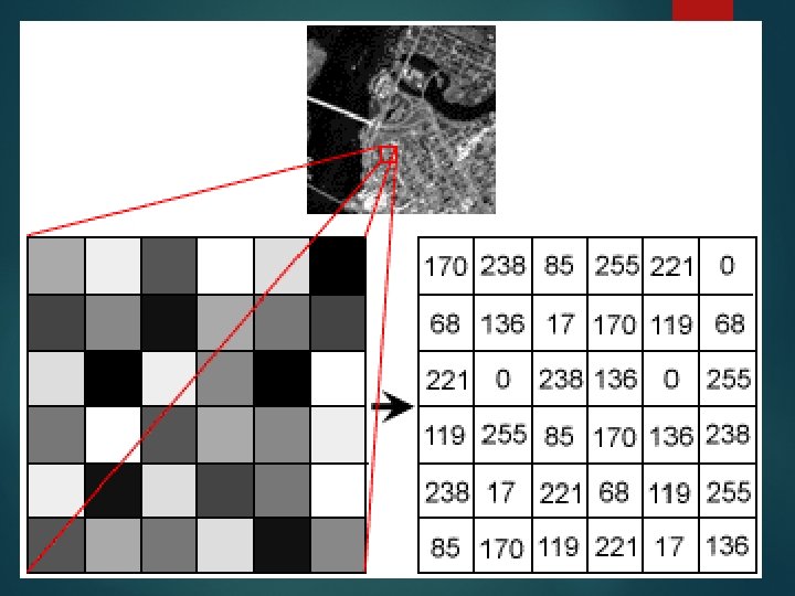
Raster Data � Imaginary matrix (row & column format) is placed over the feature (e. g. , the ground) � Some phenomenon (e. g. amount of reflected light) is measured � A value (called a digital number or DN) representing the strength of the signal (amount of light) is assigned to each grid cell (pixel).

Somewhere on earth

Overlay raster grid

Assign DNs to pixels 32 47 67 93 11 105 79 136 155 35 55 213 179 203 23 163 63 11 145 245 89 211 189 56 201 202 21 122 109 43

Image Bands � You can think of image bands (also called channels and sometimes layers) as a collection of pictures taken simultaneously of the same place, each of which measures reflected light from a different part of the spectrum. � Together, image bands allow us to create spectral curves for each pixel.

How are images stored? � Many proprietary image file formats (e. g. , Erdas Imagine) � Typically include 1) a header and 2) the image data � Image data can be organized in several ways � Band Sequential (BSQ) � Band Interleaved by Line (BIL) � Band Interleaved by Pixel (BIP) � You sometimes have to know (or guess) file structures to import images into image processing software. (Indian [IRS] data story. ) � https: //www. loc. gov/preservation/digital/formats/fdd 000420. s html � https: //gisgeography. com/gis-formats/

Example 1 1 1 2 2 2 3 3 3 1 1 2 2 3 3 1 Band 1 2 Band 2 3 bands, 9 pixels each 3 Band 3

1 1 1 1 1 2 2 2 2 2 3 3 3 3 3 Case 1 � Band sequential (BSQ) format � Band #1 is stored first � Followed � Bands by #2, #3 are stored sequentially

1 1 1 1 1 2 2 2 2 2 3 3 3 3 3 1 1 1 2 2 2 3 3 3 Case 2 � BIL format � Line #1, band #1 is stored first � Followed by line #1, band #2 � Bands are interleaved by line

1 1 1 1 1 2 2 2 2 2 3 3 3 3 3 1 2 3 1 2 3 1 2 3 Case 3 � BIP format � Pixel #1, Line #1, band #1 is stored first � Followed by Pixel #1, line #1, band #2 � Bands are interleaved by PIXEL

Histograms � A histogram is a graph showing the number of pixels in a single band corresponding to each possible DN. � Histograms give us information about the data distribution in each band (e. g. normal, skewed, bimodal, etc. ) � We use information from histograms for contrast stretching, atmospheric correction, statistical analyses, and many other applications.

# of pixels Describe the shape of this histogram.

Contrast Stretching � Computer monitors have a range of brightness that they use to display images. � Unprocessed remotely sensed images often don’t use the full range, resulting in a “washed-out” image. � Contrast stretching changes (usually temporarily) the DNs to take advantage of the full tonal range available. � Usually best not to permanently change the DNs. Why?

High Contrast Low Contrast

Types of Contrast Stretches Contrast stretches can be linear (DNs stretched evenly across the available range of values) � …or they can be nonlinear (some DNs changed more than others) � Within each of these are many different stretching algorithms. � Which you choose depends on what you are trying to see in an image. � � Erdas and other image display software often applies a temporary contrast stretch automatically to make images looks crisp.

Non-linear Contrast Stretch Linear Contrast Stretch

Laramie Landsat 8 Image Linear stretch (min-max) Standard Deviation stretch Cuts off extremes and linearly stretches remaining pixels

REMEMBER!!!!! � Contrast stretches are purely visual. You do NOT actually change any data values. � Now, let’s play with a few before lab.