Understanding Individual Markets Supply Demand CHAPTER THREE Big

Understanding Individual Markets: Supply & Demand CHAPTER THREE Big Unit Test

Test Chapter 1 - 2 - 3 • Wednesday 9/28 • Bonus work chapter 3 for Friday 9/23 Learning Supply and Demand manipulation • Essential to your Success

I. Markets • A. Defined • 1. Institution or mechanism that brings together buyers (demanders) and sellers (suppliers). • 2. Examples – Auctions, stores, stock exchanges etc… • We have already seen two markets in the simple circular flow!

A quick review • Establish whether this is in the product market or resource market. • Also establish whether it is being demanded or supplied. • 1. What is a business willing to pay a newly hired employee? • 2. What will a person buy a GHS sweatshirt for? • 3. What will a business sell a sub sandwich for? • 4. What will a person sell their property for?

MARKETS DEFINED

MARKETS DEFINED POTENTIAL BUYERS

MARKETS DEFINED POTENTIAL BUYERS POTENTIAL SELLERS

MARKETS DEFINED POTENTIAL BUYERS POTENTIAL SELLERS MARKETS

II. Demand • A. Defined • 1. Curve showing the various amounts of a product(resource) consumers(businesses) are willing and able to purchase at various prices during a specific period of time other things being equal. • 2. Demand shows us the purchasers intent with respect to the purchase of a product. • “ I would be willing to pay $1 for a Reeses Peanut Butter cup. ”

DEMAND DEFINED Demand: üWant it! ü Be able to purchase it!! ü Make the purchase!!!

DEMAND DEFINED P $1 2 3 4 5 QD 80 55 35 20 10 DEMAND SCHEDULE 3. Example of Demand schedule

DEMAND DEFINED P $1 2 3 4 5 QD 80 55 35 20 10 DEMAND SCHEDULE Various Amounts

DEMAND DEFINED P $1 2 3 4 5 QD 80 55 35 20 10 DEMAND SCHEDULE Various Amounts A Series of Possible Prices …a specified time period …other things being equal

II. Demand cont… • B. Law of Demand • 1. All else equal, as the price falls the quantity demanded rises and as the price rises the quantity demanded falls. • 2. It is an inverse relationship. • (Think John Travolta’s right hand! ) • 3. Keep in mind the other things equal assumption!

LAW OF DEMAND

LAW OF DEMAND • As Price Falls…

LAW OF DEMAND • As Price Falls… …Quantity Demanded Rises

LAW OF DEMAND • As Price Falls… …Quantity Demanded Rises • As Price Rises…

LAW OF DEMAND • As Price Falls… …Quantity Demanded Rises • As Price Rises… …Quantity Demanded Falls

LAW OF DEMAND • As Price Falls… …Quantity Demanded Rises • As Price Rises… …Quantity Demanded Falls An inverse relationship exists between price and quantity demanded

II. Demand cont… • C. Foundations for the law of demand. • 1. Common sense – why do businesses put items on sale? (Kohl’s) • 2. Diminishing marginal utility – typically (Adam and Elton are exceptions) the more you purchase a good the less satisfaction or utility you will receive. You will only buy additional units if the price falls.

II. Demand cont… • 3. Income effect – a lower price increases the purchasing power of a buyers income or budget. • 4. Substitution effect – a lower price provides incentive to substitute the now cheaper good for other goods that are now more expensive.

LAW OF DEMAND • As Price Falls… …Quantity Demanded Rises • As Price Rises… …Quantity Demanded Falls An inverse relationship exists between price and quantity demanded

LAW OF DEMAND or Why Demand Curves Slope Down! • • • Diminishing Marginal Utility Income Effect Substitution Effect Demand Curve Individual and Market Demand

II. Demand cont… • D. The demand curve • 1. Graphic illustration of how demand slopes down to the right using the demand schedule. • E. Determinants of demand – shifters that will affect where the placement of the demand curve will lie. • - They are the other things equal. • - Changes in the determinants of demand will shift the entire demand curve.

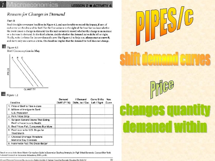
PIPES/c • • • Population Income Preference Expectations Substitutes & Complements

II. Demand cont… • F. Change in the determinants of demand that lead to a change in demand • 1. Preference or Tastes – favorable shifts to right, unfavorable shifts to left.

II. Demand cont… • 2. Population – the number of buyers either increases or decreases. (Baby Boomers) • You draw what will happen • 3. Income – Higher income causes an increase in demand for normal goods. • - inferior goods may see a decline (Ramen noodles)

DETERMINANTS OF DEMAND

DETERMINANTS OF DEMAND • Tastes and Preferences

DETERMINANTS OF DEMAND • Tastes and Preferences • Number of Customers

DETERMINANTS OF DEMAND • Tastes and Preferences • Number of Customers • Money Incomes – Normal (Superior) & Inferior Goods

II. Demand cont… • 4. Substitutes and compliments – If the price of a substitute good goes up demand for the other goes up. (Pepsi or Coke). • - If the price of a compliment goes up demand for the other goes down. (gasoline and oil). • 5. Expectations – when consumers anticipate a change in price it may prompt them to buy or not buy in anticipation of the change. • - Long lines at the gas pump in anticipation of Tropical Storm Rita? • - Result?

DETERMINANTS OF DEMAND • Tastes and Preferences • Number of Customers • Money Incomes – Normal (Superior) & Inferior Goods • Prices of Related Goods – Substitutes & Complements

DETERMINANTS OF DEMAND • Tastes and Preferences • Number of Customers • Money Incomes – Normal (Superior) & Inferior Goods • Prices of Related Goods – Substitutes & Complements • Consumer Expectations

Graphing Demand Price of Corn CORN P $1 2 3 4 5 QD 80 55 35 20 10 P$5 Plot the Points 4 3 2 1 o 10 20 30 40 50 60 70 80 Quantity of Corn Q

Graphing Demand Price of Corn CORN P $1 2 3 4 5 P$5 Plot the Points QD 4 80 55 3 35 P 1 20 2 10 1 o 10 20 30 40 50 • 5560 70 80 Quantity of Corn Q

Graphing Demand Price of Corn CORN P $1 2 3 4 5 QD 80 55 35 20 10 P$5 Plot the Points 4 Etc. 3 2 1 o 10 20 30 3540 50 60 70 80 Quantity of Corn Q

Graphing Demand Price of Corn CORN P $1 2 3 4 5 QD 80 55 35 20 10 P$5 4 3 2 1 o D 10 20 30 40 50 60 70 80 Quantity of Corn Q

II. Demand cont… • G. Change in Demand versus Change in Quantity demanded. • 1. A change in demand is a shift of the entire curve based on those changes in determinants. • 2. A change in quantity demanded is movement along the same demand curve if the price changes.

Would these two AP Econ students rate Pizza the same? Would these two AP Econ students rate shoes the same? Would these two AP Econ students rate soda the same? Would these two AP Econ students rate homework the same?

II. Demand cont… • H. Consumer Surplus • 1. The additional utility an individual or group of buyers receive when they would be willing to pay a higher price along a demand curve but do not have to.

Consumer Surplus • If a slice of pizza costs $1. 50, but Jacob would pay $2. 00 for the slice of pizza than Jacob’s consumer surplus is $0. 50. • If a new pair of football shoes costs $64. 50, and Andy would pay $70. 00 for a pair of football shoes than his consumer surplus is $5. 50. • They would feel good about their lucky purchases! Both boys have received some UTILITY!

Price $40 $30 At a price of $30! $20 $10 AP Tests 2000, 2003 & 2004 & 2005 Not in our Text! In your Activity book! Quantity

D 150 50 250

D 2 D 1 D

Pg 18

Supply v Quantity Supplied • Supply is producers • Supply is stuff • Qs v S • The mind of the producer? ? ? – Price up? Good or Bad – Wages up? Good or Bad

III. Supply • A. Defined • 1. The amount of a product a producer is willing and able to produce and make available for sale at a specific period in time. • B. Law of Supply • 1. A direct relationship – as price rises quantity supplied rises. • 2. Common sense and incentive prove the relationship.

SUPPLY DEFINED CORN P $1 2 3 4 5 QD 80 55 35 20 10 SUPPLY SCHEDULE 3. Example of a supply schedule CORN P QS $1 2 3 4 5 5 20 35 50 60

SUPPLY DEFINED CORN P $1 2 3 4 5 SUPPLY SCHEDULE QD 80 Various Amounts 55 35 20 10 CORN P QS $1 2 3 4 5 5 20 35 50 60

SUPPLY DEFINED CORN P $1 2 3 4 5 SUPPLY SCHEDULE QD 80 Various Amounts 55 35 A Series of Possible Prices 20 10 …a specified time period …other things being equal CORN P QS $1 2 3 4 5 5 20 35 50 60

LAW OF SUPPLY

LAW OF SUPPLY • As Price Rises…

LAW OF SUPPLY • As Price Rises… …Quantity Supplied Rises

LAW OF SUPPLY • As Price Rises… …Quantity Supplied Rises • As Price Falls…

LAW OF SUPPLY • As Price Rises… …Quantity Supplied Rises • As Price Falls… …Quantity Supplied Falls

LAW OF SUPPLY • As Price Rises… …Quantity Supplied Rises • As Price Falls… …Quantity Supplied Falls A direct relationship exists between price and quantity supplied

III. Supply cont… • C. Changes in supply – what shifts the supply curve? • 1. Input or resource prices – (CELL) the more it costs the less incentive to produce. • 2. Technology – When technology improves it results in resources being used more efficiently and at less of a cost. • 3. Substitutes – Sometimes firms can use their facilities to produce similar goods. Higher prices of the substitute would provide incentive to change supply.

II. Supply cont… • 4. Disaster or expectations – the actual effects of a natural disaster or predictions about the future price of a product. • 5. Size of Industry – As more firms enter an industry the more supplied. • 6. Government – Taxes, subsidies and regulations. • - Taxes and regulations mean more cost less supply. • - Subsidies lower production costs and increase supply.

Supply - DIGTS • Disaster • Input Prices • Government Policies – Taxes – Subsidies – Regulations • Technology • Size • Substitutes

DETERMINANTS OF SUPPLY

DETERMINANTS OF SUPPLY • Resource Prices

DETERMINANTS OF SUPPLY • Resource Prices • Technique of Production

DETERMINANTS OF SUPPLY • Resource Prices • Technique of Production • Taxes & Subsidies

DETERMINANTS OF SUPPLY • • Resource Prices Technique of Production Taxes & Subsidies Prices of Other Goods

DETERMINANTS OF SUPPLY • • • Resource Prices Technique of Production Taxes & Subsidies Prices of Other Goods Price Expectations

DETERMINANTS OF SUPPLY • • • Resource Prices Technique of Production Taxes & Subsidies Prices of Other Goods Price Expectations Number of Sellers

Graphing Supply Price of Corn CORN P $1 2 3 4 5 QD 80 55 35 20 10 P$5 Plot the Points CORN P QS 4 $1 2 3 4 5 3 2 1 o 5 10 20 30 40 50 60 70 80 Quantity of Corn Q 5 20 35 50 60

Graphing Supply Price of Corn CORN P $1 2 3 4 5 QD 80 55 35 20 10 P$5 Plot the Points CORN P QS 4 $1 2 3 4 5 3 2 1 o 10 20 30 40 50 60 70 80 Quantity of Corn Q 5 20 35 50 60

Graphing Supply Price of Corn CORN P $1 2 3 4 5 QD 80 55 35 20 10 P$5 Plot the Points CORN P QS Etc. 4 $1 2 3 4 5 3 2 1 o 10 20 30 3540 50 60 70 80 Quantity of Corn Q 5 20 35 50 60

Graphing Supply Price of Corn CORN P $1 2 3 4 5 QD 80 55 35 20 10 P$5 S CORN P QS 4 $1 2 3 4 5 3 2 1 o 10 20 30 40 50 60 70 80 Quantity of Corn Q 5 20 35 50 60

Graphing Supply Price of Corn CORN P $1 2 3 4 5 QD 80 55 35 20 10 P$5 S P QS 4 $1 Combining 2 3 with 4 Demand 5 3 2 1 o CORN 10 20 30 40 50 60 70 80 Quantity of Corn Q 5 20 35 50 60

Demand & Supply Price of Corn CORN P $1 2 3 4 5 P$5 S P QS QD 4 80 55 P 1 3 35 20 2 10 Market $1 2 Clearing 3 Equilibrium 4 5 1 o CORN D 10 20 30 3540 Q 1 50 60 70 80 Quantity of Corn Q 5 20 35 50 60

This Week in Econ! • Prepare for unit test!!! • Finish work on Chapters 1 - 2 – 3 • Practice manipulation of Demand Supply • Learn “Price ceilings” & “Price floors” • Learn Elasticity

IV. Market Equilibrium • A. Shows how the buying decisions of households and selling decisions of businesses interact to determine price. • 1. Equilibrium or Market clearing – the price is at rest. • 2. When not at equilibrium pricing decisions will be made to bring the market into equilibrium – rationing function of prices

Consumer Surplus in Total Producer Surplus in Total P S S All buyers who would have paid a price higher than the market clearing price are happy and receive a Consumer Surplus! All sellers who would have sold at a price lower than the market clearing price are happy and receive a Producer Surplus! P AP Tests 2000 2003, & 2004 not in our Text or the AP curriculum D Q Q

3. Disequilibrium: SURPLUS P The result of imposing a Price that is too HIGH! Ph D S SURPLUS Prices above Equilibrium cause Surplus! P S Surpluses put pressure on producers to lower price!! D Qd = Qs Q

Demand & Supply Price of Corn CORN P $1 2 3 4 5 QD 80 55 35 20 10 P$5 Surplus 4 CORN P QS more is being $1 2 supplied than 3 demanded 4 5 3 2 1 o S At a $5 price D 10 20 30 40 50 60 70 80 Quantity of Corn Q 5 20 35 50 60

4. Dead Weight Loss When a Price is set P at a level above Market = The loss in satisfaction or P 2 utility of consumers and P 1 producers. S Price Floor Farm Subsidy Dairy Farmers D Q 2 Q 1 Q

5. Disequilibrium: SHORTAGE P D S P Pl S Shortages put pressure on producers to raise price!! SHORTAGE Qs = Qd D Q

6. Dead Weight Loss When the price is set below P Market= A loss in Satisfaction or utility of consumers and producers. S D Price Ceiling Rent Control P 1 A Maximum Price P 2 S D Qs Q 1 Qd Q

Demand & Supply Price of Corn CORN P $1 2 3 4 5 QD 80 55 35 20 10 P$5 S At a $1 price 4 P QS more is being $1 2 demanded than 3 supplied 4 5 Shortage 3 2 1 o CORN D 10 20 30 40 50 60 70 80 Quantity of Corn Q 5 20 35 50 60

P True Market Price! Deadweight Loss When a Product is Taxed Excise Tax s + Tax S New market price paid by consumers Dead Weight Loss From 2003 Essay! Free Market Price too Low! Amount of Tax needed to correct Negative externality! D 0 Copyright Schill 2004! Qd = Q s Over allocation – too much bad stuff Q

Demand & Supply Price of Corn CORN P $1 2 3 4 5 P$5 S P QS QD 4 80 55 P 1 3 35 20 2 10 Market $1 2 Clearing 3 Equilibrium 4 5 1 o CORN D 10 20 30 3540 Q 1 50 60 70 80 Quantity of Corn Q 5 20 35 50 60

Demand & Supply Price of Corn P$5 S What if Demand Increases? 4 3 2 1 o D 10 20 30 40 50 60 70 80 Quantity of Corn Q

Demand & Supply Price of Corn P$5 S Increase in Quantity Supplied Increase in Demand 4 3 2 D’ 1 o D 10 20 30 40 50 60 70 80 Quantity of Corn Q

Demand & Supply Price of Corn P$5 S What if Demand Decreases? 4 3 2 D’ 1 o D 10 20 30 40 50 60 70 80 Quantity of Corn Q

Demand & Supply Price of Corn Decrease in Quantity Supplied P$5 4 3 S Decrease in Demand 2 1 o D’ 10 20 30 40 50 60 70 80 Quantity of Corn D Q

Demand & Supply Price of Corn P$5 S What if Supply Increases? 4 3 2 1 o D 10 20 30 40 50 60 70 80 Quantity of Corn Q

Demand & Supply Price of Corn P$5 Increase in Supply 4 S S’ Increase in Quantity Demanded 3 2 1 o D 10 20 30 40 50 60 70 80 Quantity of Corn Q

Demand & Supply Price of Corn P$5 S What if Supply Decreases? 4 3 2 S’ 1 o D 10 20 30 40 50 60 70 80 Quantity of Corn Q

Demand & Supply Decrease S’ Price of Corn P$5 in Supply S 4 Decrease in Quantity Demanded 3 2 1 o D 10 20 30 40 50 60 70 80 Quantity of Corn Q

What if both demand supply increase? What if both demand supply decrease? P S 1 S 2 P 2? P 1 D 1 Q 2 D 2 Q

V. Elasticity • A. Demand • 1. If consumers are highly responsive to price changes the demand curve is ELASTIC. • 2. Example farmers market – if there is any price difference among tomato growers, you don’t buy or have any demand because there are so many alternatives available to you.

Perfectly Elastic Demand Curve P Tomatoes $1. 50? ? p 1 d 1 s 1 Tomatoes $1. 00 s 2 Q Because there are so many alternatives there will be no demand at a higher price.

V. Elasticity cont… • 3. If consumers are not responsive at all to price changes their demand curve is INELASTIC. • 4. Example – diabetics demand for insulin. No matter what the cost they still must have the good.

Perfectly Inelastic Demand Curve P s 2 s 1 d 1 Need it no matter what the price Q

V. Elasticity cont… • B. Supply • 1. Perfectly INELASTIC cannot change the amount supplied in the short term • 2. Example Bradley Center.

Perfectly Inelastic Supply P S d 2 d 1 Q Short term – difficult to alter supply so a larger impact on price.

V. Elasticity cont… • 3. Elastic supply – the more a supplier can transfer resources to produce more of a good the more elastic supply. • 4. Example - farmers converting land to produce more of a product that sees a price increase.

Elastic Supply P S d 2 d 1 Q The more time goes on and resources can be transferred the more elastic supply. Reflected in a smaller price change.

Signals Graphs

The Product Market Individual Firms S Households Signals D

Individual Firm Product Market Household s = MC S P* d = MR q* P* Q* P* s D d q* The Product Market signals both Households and Individual Firm the price of products. The signals indicate P* to both. Based on its cost of producing one more firms determine how much. Based on their demand consumer determine how many.

Workers Factor Market Labor Individual Firms s = MSC S P* d = MSB P* MRC P* MRP D q* Q* q* The Factor Market signals both Workers and Individual Firms the price of labor & the wage of labor. The signals indicate P* to both. Based on its revenue/worker(mrp) vs. its costs(mrc) firms determine how many workers to hire (mrp=mrc). Based on their Marginal Benefit vs. Marginal Cost workers determine whether or not they will work for this wage (msc=msb).

Market Equilibrium

Market Equilibrium • Equilibrium Price & Quantity

Market Equilibrium • Equilibrium Price & Quantity • Rationing Function of Prices

Market Equilibrium • Equilibrium Price & Quantity • Rationing Function of Prices • Changes in Demand

Market Equilibrium • • Equilibrium Price & Quantity Rationing Function of Prices Changes in Demand Changes in Quantity Demanded

Market Equilibrium • • • Equilibrium Price & Quantity Rationing Function of Prices Changes in Demand Changes in Quantity Demanded Changes in Supply

What is on the Unit 1 Test? Unlimited Wants Satisfied by Limited Resources

Limited vs Unlimited • Little kids & parents in a store…. “but I want it now!” • Teenagers & parents on a weekend… “but all my friends are going!” Unlimited wants v Limited Resources


Economics, the study of choice!

Making a Choice Carries a Cost! • Opportunity Cost • When one road is taken an opportunity on another road is missed! • In taking AP Econ, what did you not take? • Going out for a sport means…. . • Buying a new outfit means…. .

3 Basic Questions for any nation: 1. What? 2. How? 3. For Whom? To answer these questions, economic systems were created.

Economic Systems • • Traditional Command Market Mixed Each system answers: what, how, and for whom differently.

THE FOUNDATION OF ECONOMICS SOCIETY HAS VIRTUALLY UNLIMITED WANTS. . BUT LIMITED OR SCARCE PRODUCTIVE RESOURCES!

Circular Flow Model $ COSTS $ INCOMES RESOURCE MARKET RESOURCES INPUTS BUSINESSES HOUSEHOLDS GOODS & SERVICES PRODUCT MARKET $ REVENUE $ CONSUMPTION

PRODUCTION POSSIBILITIES Capital Goods Q A a Economic Limits Along PPC Frontier B Consumer Goods Q

PRODUCTION POSSIBILITIES Capital Goods Q Economic Growth C A b a B D Consumer Goods Q

The Role of Government FULL EMPLOYMENT STABLE PRICES ECONOMIC GROWTH ALLOCATIVE EFFICIENCY PRODUCTIVE EFFICIENCY
 Q 14 13 12 11 A B 10 C 9")
PRODUCTION POSSIBILITIES Robots (thousands) Q 14 13 12 11 A B 10 C 9 8 7 D 6 5 Attainable 4 but 3 2 Inefficient 1 1 2 3 Unattainable W Attainable and efficient E 4 5 6 7 Pizzas (hundred thousands) 8 Q
 Q 14 Unemployment & Underemployment Shown by Point U 13")
PRODUCTION POSSIBILITIES Robots (thousands) Q 14 Unemployment & Underemployment Shown by Point U 13 12 11 10 9 8 7 6 5 4 3 2 1 More of either or both is possible U 1 2 3 4 5 6 7 Pizzas (hundred thousands) 8 Q

Market Equilibrium • • • Equilibrium Price & Quantity Rationing Function of Prices Changes in Demand Changes in Quantity Demanded Changes in Supply Changes in Quantity Supplied

Demand v Quantity Demanded • Demand is Consumers • Demand is Feelings • Qd v D • The mind of the buyer? ? ? – Price up? Good or Bad – Income up? Good or Bad

PIPES/c • • • Population Income Preference Expectations Substitutes & Compliments

Supply v Quantity Supplied • Supply is producers • Supply is stuff • Qs v S • The mind of the producer? ? ? – Price up? Good or Bad – Wages up? Good or Bad

Supply - DIGTS • Disaster • Input Prices • Government Policies – Taxes – Subsidies – Regulations • Technology • Size of Industry • Substitutes

Market Disequilibrium! • Price Floors: Minimum Wage, Farm Price Supports • Surplus • Price Ceilings: Rent Controls • Shortages • Producer and Consumer Surplus

Applications. . . Price Ceiling P D S The result of imposing a legal price ceiling is a. . . P S D Q

Applications. . . Price Ceiling P D P Pc Legal Price Ceiling S Example: Rent Controls S SHORTAGE D Q

Applications. . . Price Ceiling P D S With shortages comes. . . Rationing Problems and P Legal Price Ceiling Black Markets Pc S SHORTAGE D Q

Applications. . . Price Ceiling Rent Controls

Applications. . . Price Ceiling Rent Controls Credit Card Interest Ceilings

Applications. . . Price Ceiling Rent Controls Credit Card Interest Ceilings

Applications. . . The result of imposing a legal price floor is a. . . P D S P S D Q Q

Applications. . . P The result of imposing a legal price floor is a. . . Pf D S SURPLUS Legal Price Floor P S Minimum Wage – Farm Support Prices D Qd Q Qs Q

Consumer Surplus in Total Producer Surplus in Total P S S Allsellers buyers who would have All who would have paid than the sold at aa price higher lower than market clearing price are the market clearing price happy and receive aa are happy and receive Consumer Surplus! Producer Surplus! P AP Tests 2000 & 2003 not in our Text or the AP curriculum D Q Q

Dead Weight Loss P S Price Floor P 2 P 1 D Q 2 Q 1 Q

Market Equilibrium • • • Equilibrium Price & Quantity Rationing Function of Prices Complex Cases Changes in Demand Multiple Shifts Changes in Quantity Demanded Changes in Supply Changes in Quantity Supplied

Market Equilibrium • • • Equilibrium Price & Quantity Rationing Function of Prices Chapter Changes in Demand Conclusion Changes in Quantity Demanded Changes in Supply Changes in Quantity Supplied

• • • Key Terms • market demand schedule demand curve law of demand diminishing marginal utility income effects substitution effects determinants of demand normal good inferior good substitute good complementary good • • change in demand vs. quantity demanded change in supply vs. quantity supplied supply schedule determinants of supply surplus shortage equilibrium price and quantity rationing function of prices

Next: and the Chapter 4
- Slides: 149