Understanding Data Digital Audio Processing with Python Part

Understanding Data Digital Audio Processing with Python Part 2: The Discrete Fourier Transform

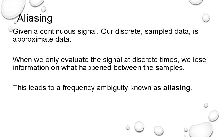
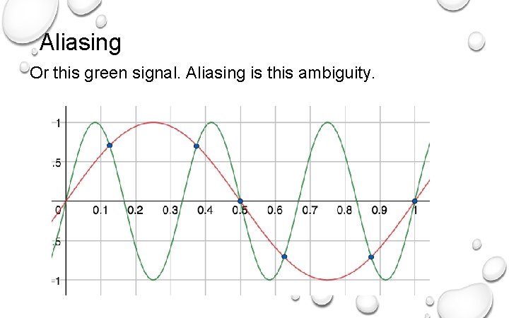
Aliasing Given a continuous signal. Our discrete, sampled data, is approximate data. When we only evaluate the signal at discrete times, we lose information on what happened between the samples. This leads to a frequency ambiguity known as aliasing.

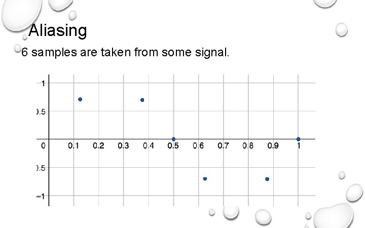
Aliasing 6 samples are taken from some signal.

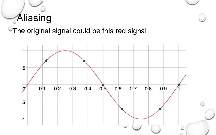
Aliasing The original signal could be this red signal.

Aliasing Or this green signal. Aliasing is this ambiguity.

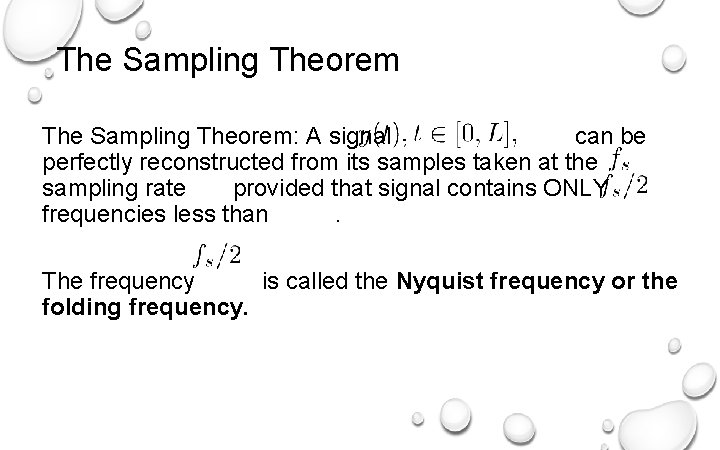
The Sampling Theorem: A signal can be perfectly reconstructed from its samples taken at the sampling rate provided that signal contains ONLY frequencies less than. The frequency is called the Nyquist frequency or the folding frequency.

Why 44100 Hz? Range of human hearing is between 20 Hz and 20, 000 Hz. To guarantee that every frequency in this range is properly recorded, the Sampling Theorem states that a sampling rate of at least 40, 000 Hz is necessary. CD quality standard sampling rate is 44100 Hz. Before sampling is taken, a lowpass-filter is applied to remove all frequencies outside of the Nyquist frequency range. This prevents aliasing and corruption of the recording. These lowpassfilters are also called anti-aliasing filters.

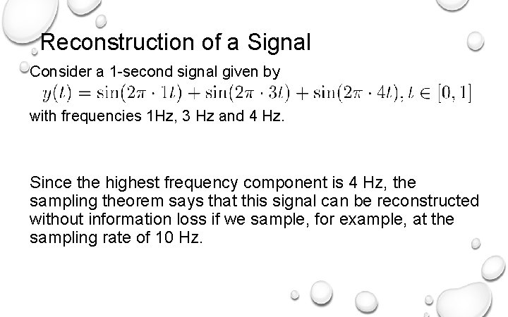
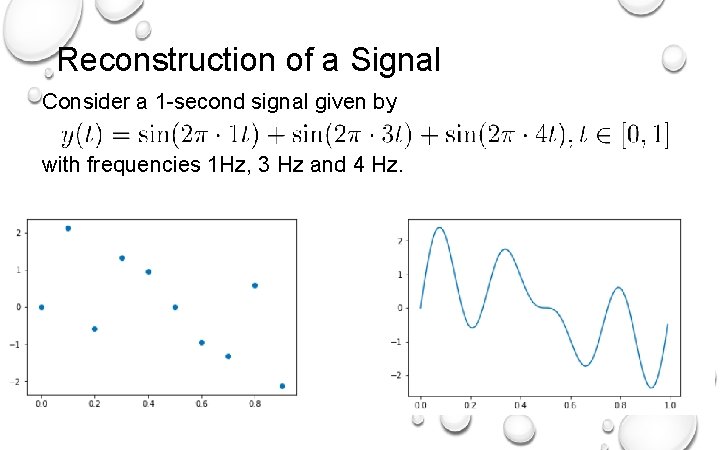
Reconstruction of a Signal Consider a 1 -second signal given by with frequencies 1 Hz, 3 Hz and 4 Hz. Since the highest frequency component is 4 Hz, the sampling theorem says that this signal can be reconstructed without information loss if we sample, for example, at the sampling rate of 10 Hz.

Reconstruction of a Signal Consider a 1 -second signal given by with frequencies 1 Hz, 3 Hz and 4 Hz.

Fundamental Frequency Consider the interval [0, L] measured in seconds. Define the frequency This frequency is called the fundamental frequency for the interval [0, L]. A sinusoid with frequency completes one cycle in the interval [0, L]. Note that since , we also have. 0 L

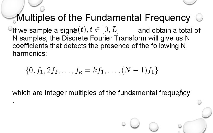
Multiples of the Fundamental Frequency If we sample a signal and obtain a total of N samples, the Discrete Fourier Transform will give us N coefficients that detects the presence of the following N harmonics: which are integer multiples of the fundamental frequency.

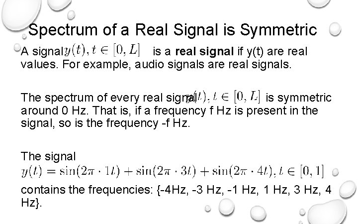
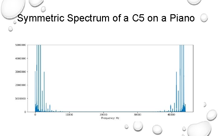
Spectrum of a Real Signal is Symmetric A signal is a real signal if y(t) are real values. For example, audio signals are real signals. The spectrum of every real signal is symmetric around 0 Hz. That is, if a frequency f Hz is present in the signal, so is the frequency -f Hz. The signal contains the frequencies: {-4 Hz, -3 Hz, -1 Hz, 3 Hz, 4 Hz}.

Symmetric Spectrum of a C 5 on a Piano

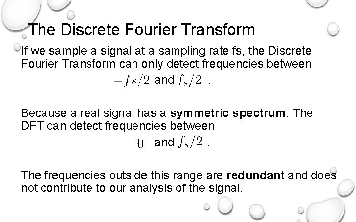
The Discrete Fourier Transform If we sample a signal at a sampling rate fs, the Discrete Fourier Transform can only detect frequencies between and. Because a real signal has a symmetric spectrum. The DFT can detect frequencies between and. The frequencies outside this range are redundant and does not contribute to our analysis of the signal.

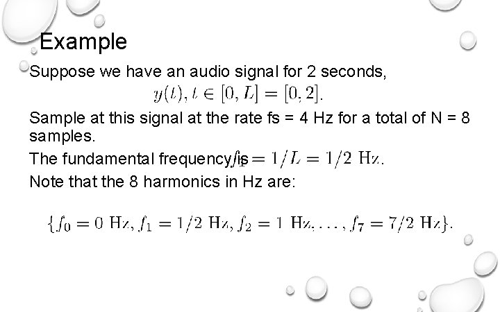
Example Suppose we have an audio signal for 2 seconds, . Sample at this signal at the rate fs = 4 Hz for a total of N = 8 samples. The fundamental frequency is. Note that the 8 harmonics in Hz are:

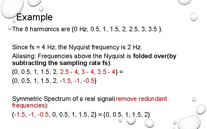
Example The 8 harmonics are {0 Hz, 0. 5, 1, 1. 5, 2, 2. 5, 3, 3. 5 }. Since fs = 4 Hz, the Nyquist frequency is 2 Hz. Aliasing: Frequencies above the Nyquist is folded over(by subtracting the sampling rate fs). {0, 0. 5, 1, 1. 5, 2, 2. 5 - 4, 3. 5 - 4} = {0, 0. 5, 1, 1. 5, 2, -1. 5, -1, -0. 5} Symmetric Spectrum of a real signal(remove redundant frequencies): {-1. 5, -1, -0. 5, 0, 0. 5, 1, 1. 5, 2} = {0, 0. 5, 1, 1. 5, 2}

The Discrete Fourier Transform

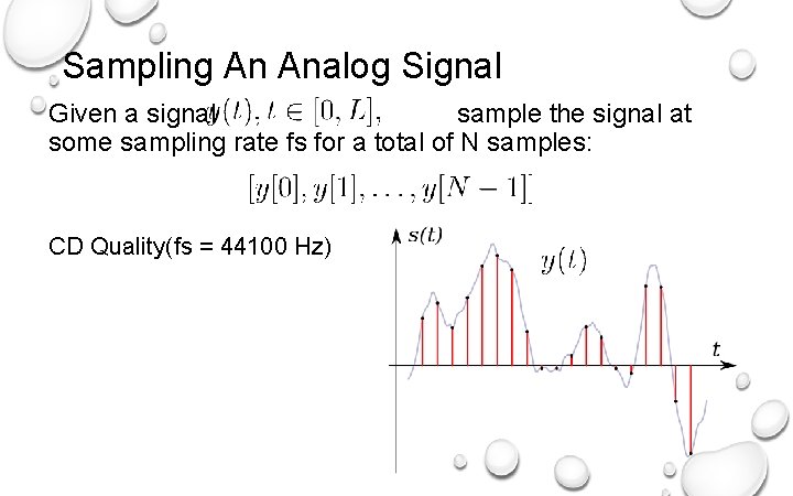
Sampling An Analog Signal Given a signal sample the signal at some sampling rate fs for a total of N samples: CD Quality(fs = 44100 Hz)

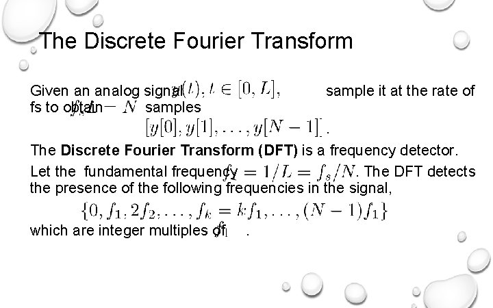
The Discrete Fourier Transform Given an analog signal fs to obtain samples sample it at the rate of . The Discrete Fourier Transform (DFT) is a frequency detector. Let the fundamental frequency. The DFT detects the presence of the following frequencies in the signal, which are integer multiples of .

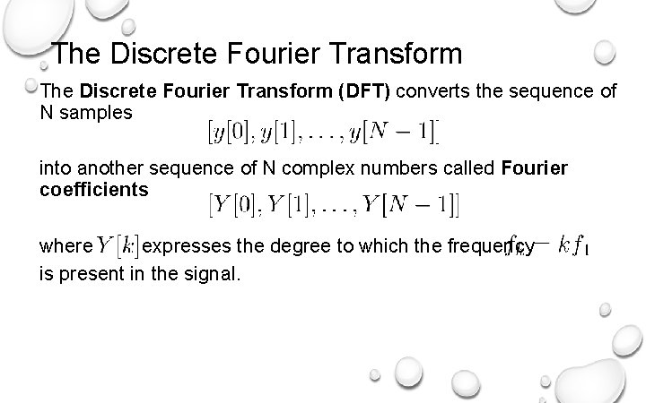
The Discrete Fourier Transform (DFT) converts the sequence of N samples into another sequence of N complex numbers called Fourier coefficients where expresses the degree to which the frequency is present in the signal.

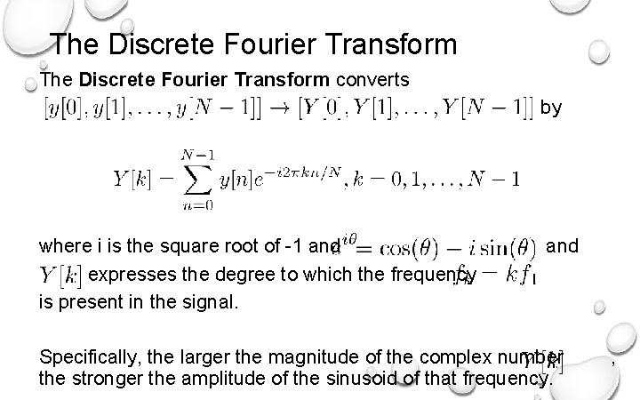
The Discrete Fourier Transform converts by where i is the square root of -1 and expresses the degree to which the frequency is present in the signal. and Specifically, the larger the magnitude of the complex number the stronger the amplitude of the sinusoid of that frequency. ,

The Discrete Fourier Transform A simplementation of the DFT uses a for loop to sum a termby-term product between the sample and the exponential to compute each Fourier coefficient. To compute all coefficients, one can use a nested set of for loops, one for each coefficient. However, such an implementation is VERY slow. The Fast Fourier Transform is a fast implementation for computing the DFT. Because of its many applications, the Fast Fourier Transform is considered one of the Top 10 Algorithms of 20 th Century by the IEEE magazine Computing in Science & Engineering.

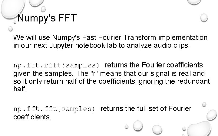
Numpy's FFT We will use Numpy's Fast Fourier Transform implementation in our next Jupyter notebook lab to analyze audio clips. np. fft. rfft(samples) returns the Fourier coefficients given the samples. The "r" means that our signal is real and so it only return half of the coefficients ignoring the redundant half. np. fft(samples) returns the full set of Fourier coefficients.

References 1) Müller, Meinard, Fundamentals of Music Processing, Springer 2015. 2) Downey, Allen, Think. DSP, Green Tea Press 2012. 3) Smith, Julius, The Mathematics of the Discrete Fourier Transform, W 3 K Publishing 2007. 4) Loy, Gareth, Musimathics, Volumes 1 and 2. The MIT Press 2011. 5) Newman, Mark, Computational Physics, Createspace Independent Publishing Platform 2012. 6) Soklaski, Ryan. MIT Lincoln Lab Researcher. Beaver Works Summer Institute.