Understanding Data Digital Audio Processing with Python Part

Understanding Data Digital Audio Processing with Python Part 1: Audio Basics

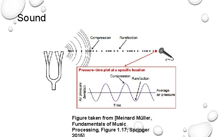
Sound Figure taken from [Meinard Müller, Fundamentals of Music Processing, Figure 1. 17, Springer

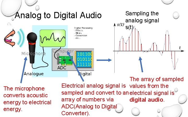
Analog to Digital Audio The microphone converts acoustic energy to electrical energy. Sampling the analog signal s(t) The array of sampled Electrical analog signal is values from the sampled and convert to an electrical signal is array of numbers via digital audio. ADC(Analog to Digital Converter).

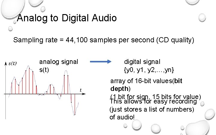
Analog to Digital Audio Sampling rate = 44, 100 samples per second (CD quality) analog signal s(t) digital signal {y 0, y 1, y 2, …, yn} array of 16 -bit values(bit depth) (1 bit for sign, 15 bits for value) This allows for easy recording (just stores a list of numbers) of audio!

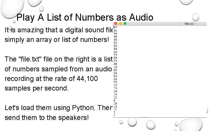
Play A List of Numbers as Audio It is amazing that a digital sound file is simply an array or list of numbers! The "file. txt" file on the right is a list of numbers sampled from an audio recording at the rate of 44, 100 samples per second. Let's load them using Python. Then send them to the speakers!

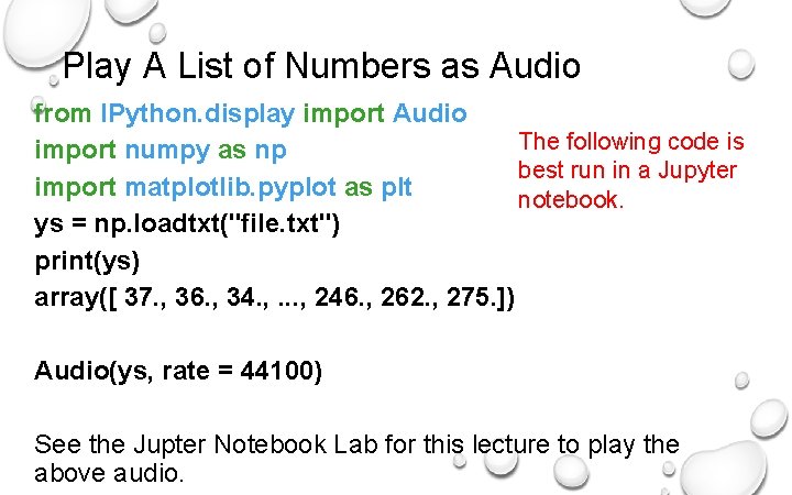
Play A List of Numbers as Audio from IPython. display import Audio The following code is import numpy as np best run in a Jupyter import matplotlib. pyplot as plt notebook. ys = np. loadtxt("file. txt") print(ys) array([ 37. , 36. , 34. , . . . , 246. , 262. , 275. ]) Audio(ys, rate = 44100) See the Jupter Notebook Lab for this lecture to play the above audio.

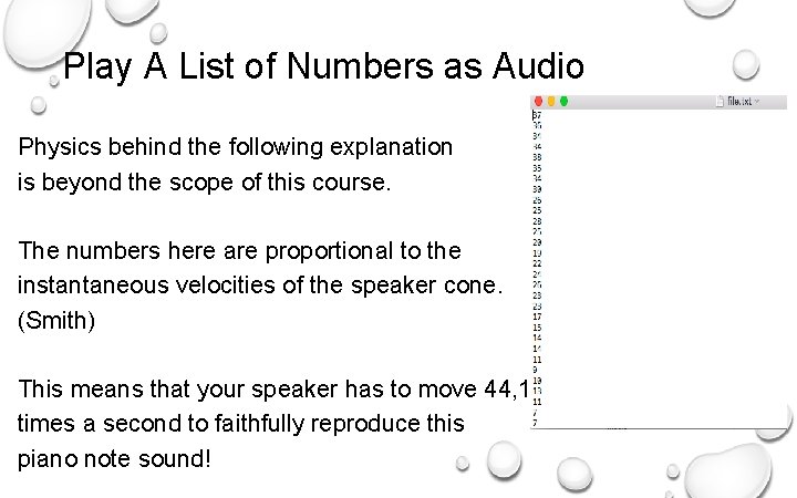
Play A List of Numbers as Audio Physics behind the following explanation is beyond the scope of this course. The numbers here are proportional to the instantaneous velocities of the speaker cone. (Smith) This means that your speaker has to move 44, 100 times a second to faithfully reproduce this piano note sound!

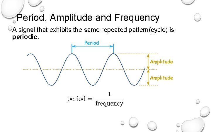
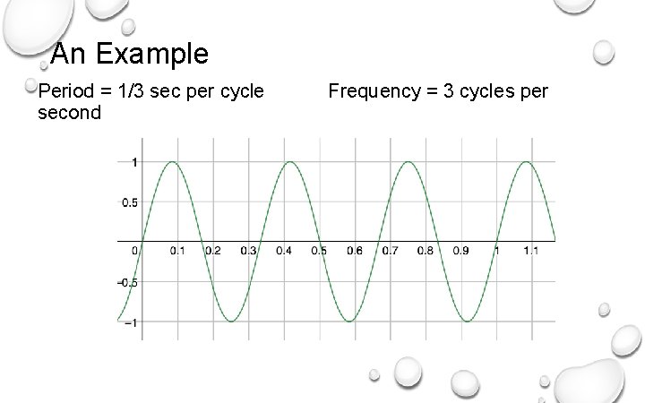
Period, Amplitude and Frequency A signal that exhibits the same repeated pattern(cycle) is periodic.

An Example Period = 1/3 sec per cycle second Frequency = 3 cycles per

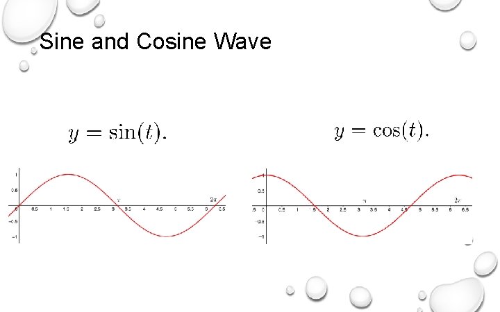
Sine and Cosine Wave

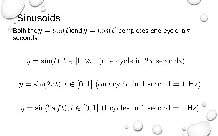
Sinusoids Both the seconds: and completes one cycle in

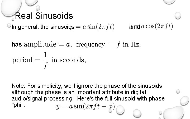
Real Sinusoids In general, the sinusoids and has Note: For simplicity, we'll ignore the phase of the sinusoids although the phase is an important attribute in digital audio/signal processing. Here's the full sinusoid with phase "phi":

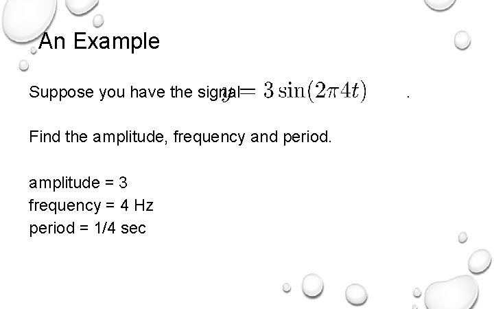
An Example Suppose you have the signal Find the amplitude, frequency and period. amplitude = 3 frequency = 4 Hz period = 1/4 sec .

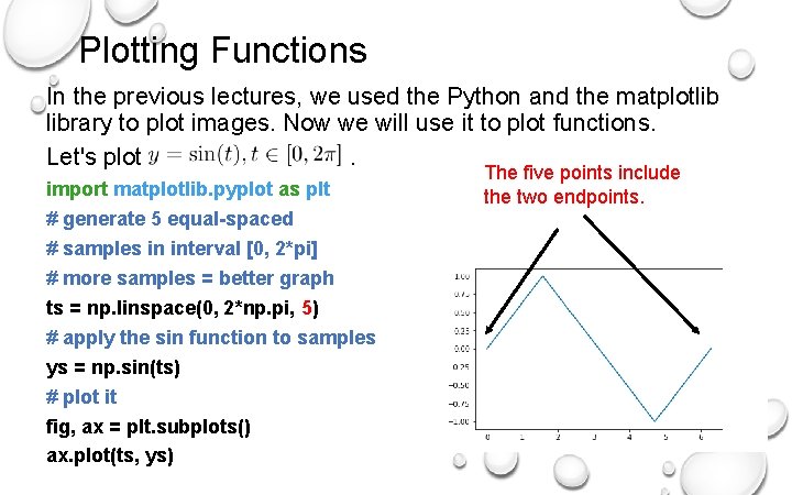
Plotting Functions In the previous lectures, we used the Python and the matplotlib library to plot images. Now we will use it to plot functions. Let's plot. import matplotlib. pyplot as plt # generate 5 equal-spaced # samples in interval [0, 2*pi] # more samples = better graph ts = np. linspace(0, 2*np. pi, 5) # apply the sin function to samples ys = np. sin(ts) # plot it fig, ax = plt. subplots() ax. plot(ts, ys) The five points include the two endpoints.

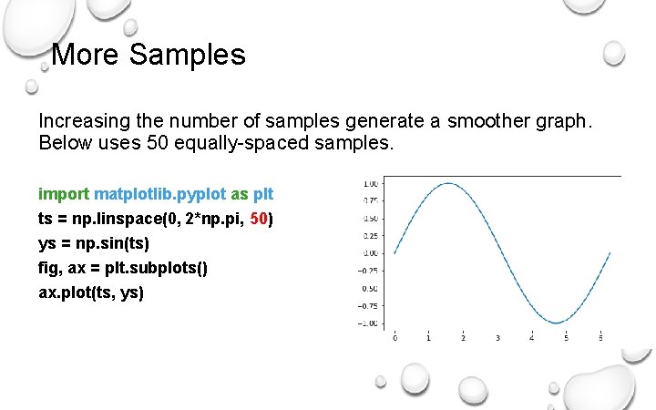
More Samples Increasing the number of samples generate a smoother graph. Below uses 50 equally-spaced samples. import matplotlib. pyplot as plt ts = np. linspace(0, 2*np. pi, 50) ys = np. sin(ts) fig, ax = plt. subplots() ax. plot(ts, ys)

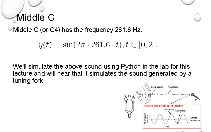
Middle C (or C 4) has the frequency 261. 6 Hz. We'll simulate the above sound using Python in the lab for this lecture and will hear that it simulates the sound generated by a tuning fork.

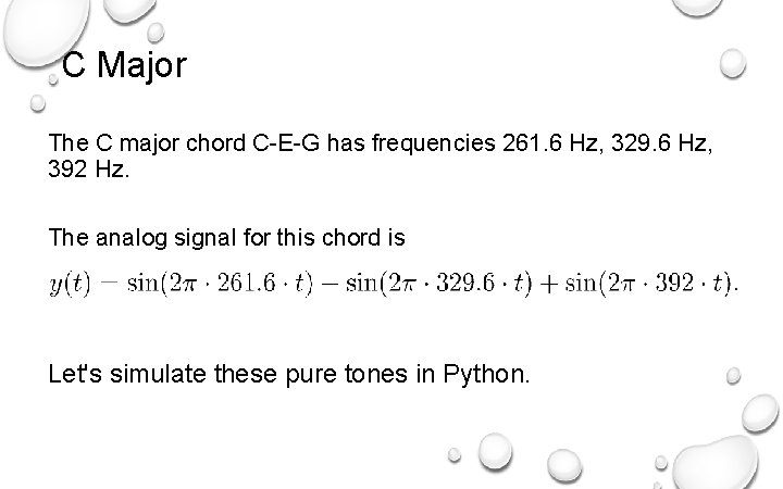
C Major The C major chord C-E-G has frequencies 261. 6 Hz, 329. 6 Hz, 392 Hz. The analog signal for this chord is Let's simulate these pure tones in Python.

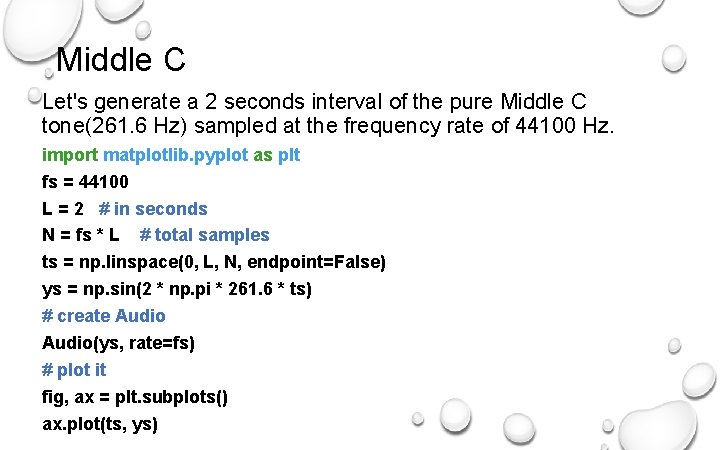
Middle C Let's generate a 2 seconds interval of the pure Middle C tone(261. 6 Hz) sampled at the frequency rate of 44100 Hz. import matplotlib. pyplot as plt fs = 44100 L = 2 # in seconds N = fs * L # total samples ts = np. linspace(0, L, N, endpoint=False) ys = np. sin(2 * np. pi * 261. 6 * ts) # create Audio(ys, rate=fs) # plot it fig, ax = plt. subplots() ax. plot(ts, ys)

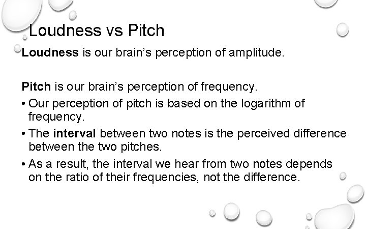
Loudness vs Pitch Loudness is our brain’s perception of amplitude. Pitch is our brain’s perception of frequency. • Our perception of pitch is based on the logarithm of frequency. • The interval between two notes is the perceived difference between the two pitches. • As a result, the interval we hear from two notes depends on the ratio of their frequencies, not the difference.

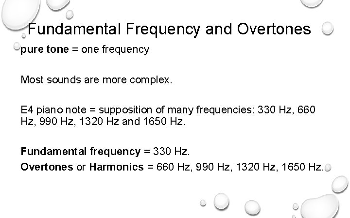
Fundamental Frequency and Overtones pure tone = one frequency Most sounds are more complex. E 4 piano note = supposition of many frequencies: 330 Hz, 660 Hz, 990 Hz, 1320 Hz and 1650 Hz. Fundamental frequency = 330 Hz. Overtones or Harmonics = 660 Hz, 990 Hz, 1320 Hz, 1650 Hz.

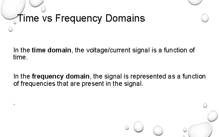
Time vs Frequency Domains In the time domain, the voltage/current signal is a function of time. In the frequency domain, the signal is represented as a function of frequencies that are present in the signal. .

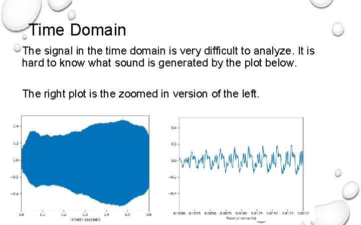
Time Domain The signal in the time domain is very difficult to analyze. It is hard to know what sound is generated by the plot below. The right plot is the zoomed in version of the left.

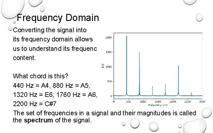
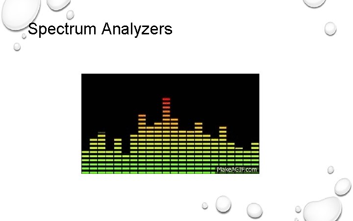
Frequency Domain Converting the signal into its frequency domain allows us to understand its frequency content. What chord is this? 440 Hz = A 4, 880 Hz = A 5, 1320 Hz = E 6, 1760 Hz = A 6, 2200 Hz = C#7 The set of frequencies in a signal and their magnitudes is called the spectrum of the signal.

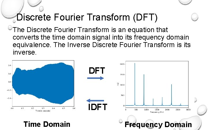
Discrete Fourier Transform (DFT) The Discrete Fourier Transform is an equation that converts the time domain signal into its frequency domain equivalence. The Inverse Discrete Fourier Transform is its inverse. DFT IDFT Time Domain Frequency Domain

Spectrum Analyzers

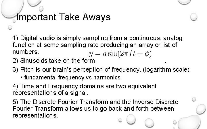
Important Take Aways 1) Digital audio is simply sampling from a continuous, analog function at some sampling rate producing an array or list of numbers. 2) Sinusoids take on the form. 3) Pitch is our brain’s perception of frequency. (logarithm scale) • fundamental frequency vs harmonics 4) Time and Frequency domains are two equivalent representations of a signal. 5) The Discrete Fourier Transform and the Inverse Discrete Fourier Transform allows us to go back and forth between representations.

Labs Download the Jupyter Notebook from my website and work through the problems.

References 1) Müller, Meinard, Fundamentals of Music Processing, Springer 2015. 2) Downey, Allen, Think. DSP, Green Tea Press 2012. 3) Smith, Julius, The Mathematics of the Discrete Fourier Transform, W 3 K Publishing 2007. 4) Loy, Gareth, Musimathics, Volumes 1 and 2. The MIT Press 2011. 5) Newman, Mark, Computational Physics, Createspace Independent Publishing Platform 2012. 6) Soklaski, Ryan. MIT Lincoln Lab Researcher. Beaver Works Summer Institute.