Under the hood Query Optimization Query Execution plans

+ Under the hood: Query Optimization, Query Execution plans

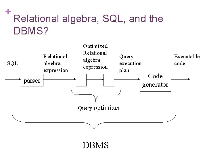
+ Relational algebra, SQL, and the DBMS? Relational algebra expression SQL Optimized Relational algebra expression Query execution plan parser Query optimizer DBMS Executable code Code generator

+ Introduction n Alternative ways of evaluating a given query n Equivalent expressions n Different algorithms for each operation n Cost difference between a good and a bad way of evaluating a query can be enormous n Need to estimate the cost of operations n n Statistical information about relations. Examples: n number of tuples, n number of distinct values for an attributes, etc. Statistics estimation for intermediate results n to compute cost of complex expressions

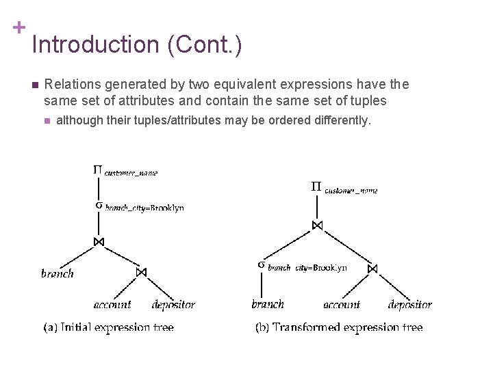
+ Introduction (Cont. ) n Relations generated by two equivalent expressions have the same set of attributes and contain the same set of tuples n although their tuples/attributes may be ordered differently.

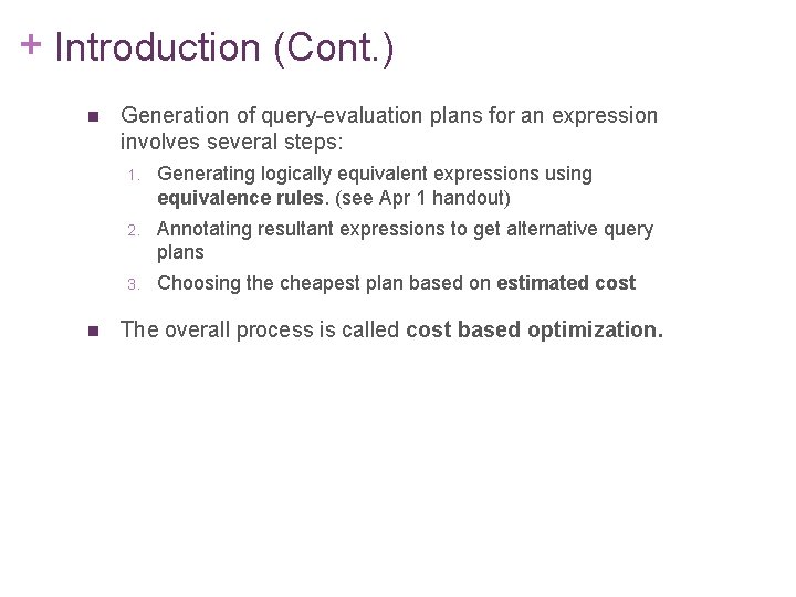
+ Introduction (Cont. ) n n Generation of query-evaluation plans for an expression involves several steps: 1. Generating logically equivalent expressions using equivalence rules. (see Apr 1 handout) 2. Annotating resultant expressions to get alternative query plans 3. Choosing the cheapest plan based on estimated cost The overall process is called cost based optimization.

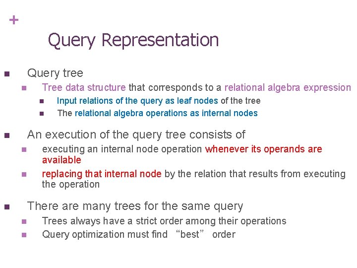
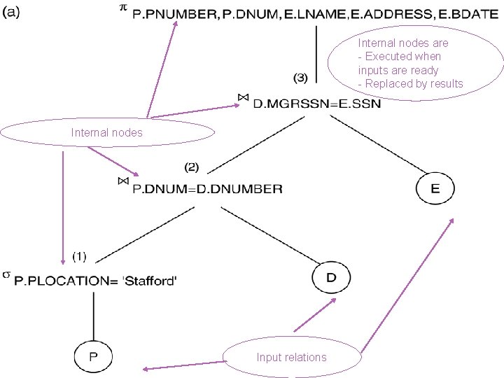
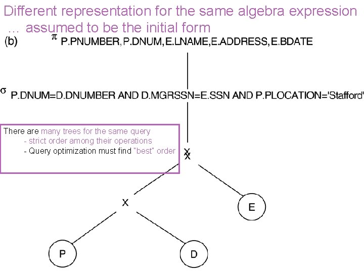
+ Query Representation Query tree n n Tree data structure that corresponds to a relational algebra expression n n Input relations of the query as leaf nodes of the tree The relational algebra operations as internal nodes An execution of the query tree consists of n n n executing an internal node operation whenever its operands are available replacing that internal node by the relation that results from executing the operation There are many trees for the same query n n n Trees always have a strict order among their operations Query optimization must find “best” order

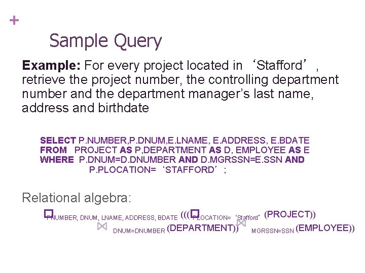
+ Sample Query Example: For every project located in‘Stafford’, retrieve the project number, the controlling department number and the department manager’s last name, address and birthdate SELECT P. NUMBER, P. DNUM, E. LNAME, E. ADDRESS, E. BDATE FROM PROJECT AS P, DEPARTMENT AS D, EMPLOYEE AS E WHERE P. DNUM=D. DNUMBER AND D. MGRSSN=E. SSN AND P. PLOCATION=‘STAFFORD’; Relational algebra: � PNUMBER, DNUM, LNAME, ADDRESS, BDATE (((� PLOCATION=‘Stafford’(PROJECT)) DNUM=DNUMBER (DEPARTMENT)) MGRSSN=SSN (EMPLOYEE))

Internal nodes are - Executed when inputs are ready - Replaced by results Internal nodes Input relations

Different representation for the same algebra expression … assumed to be the initial form There are many trees for the same query - strict order among their operations - Query optimization must find “best” order

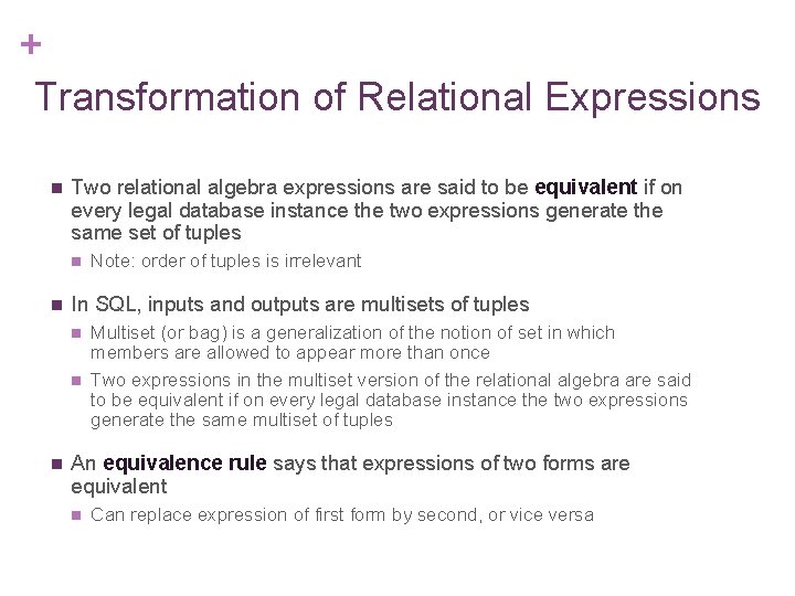
+ Transformation of Relational Expressions n Two relational algebra expressions are said to be equivalent if on every legal database instance the two expressions generate the same set of tuples n n In SQL, inputs and outputs are multisets of tuples n n n Note: order of tuples is irrelevant Multiset (or bag) is a generalization of the notion of set in which members are allowed to appear more than once Two expressions in the multiset version of the relational algebra are said to be equivalent if on every legal database instance the two expressions generate the same multiset of tuples An equivalence rule says that expressions of two forms are equivalent n Can replace expression of first form by second, or vice versa

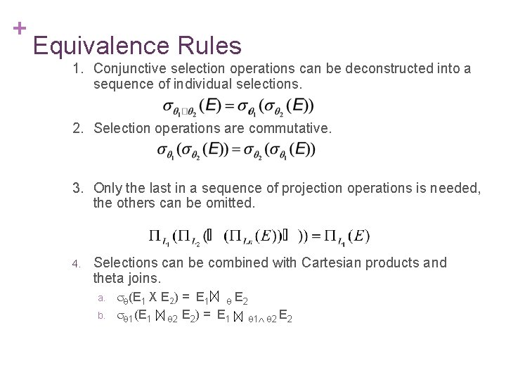
+ Equivalence Rules 1. Conjunctive selection operations can be deconstructed into a sequence of individual selections. 2. Selection operations are commutative. 3. Only the last in a sequence of projection operations is needed, the others can be omitted. 4. Selections can be combined with Cartesian products and theta joins. a. b. (E 1 X E 2) = E 1 E 2 1(E 1 2 E 2) = E 1 1 2 E 2

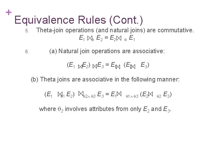
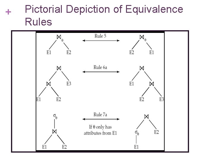
+ Equivalence Rules (Cont. ) 5. 6. Theta-join operations (and natural joins) are commutative. E 1 E 2 = E 2 E 1 (a) Natural join operations are associative: (E 1 E 2 ) E 3 = E 1 (E 2 E 3) (b) Theta joins are associative in the following manner: (E 1 1 E 2) 2 3 E 3 = E 1 1 3 (E 2 2 E 3) where 2 involves attributes from only E 2 and E 3.

+ Pictorial Depiction of Equivalence Rules

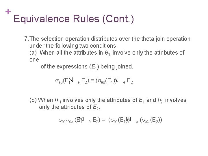
+ Equivalence Rules (Cont. ) 7. The selection operation distributes over theta join operation under the following two conditions: (a) When all the attributes in 0 involve only the attributes of one of the expressions (E 1) being joined. 0 E 1 E 2) = ( 0(E 1)) E 2 (b) When 1 involves only the attributes of E 1 and 2 involves only the attributes of E 2. 1 E 2) = ( 1(E 1)) ( (E 2))

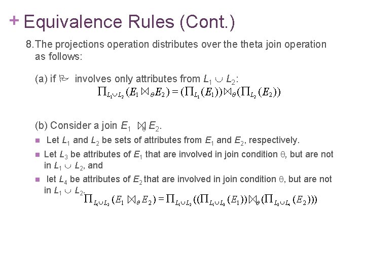
+ Equivalence Rules (Cont. ) 8. The projections operation distributes over theta join operation as follows: (a) if involves only attributes from L 1 L 2: L 1 L 2 ( E 1 (b) Consider a join E 1 n E 2 ) = ( L 1 ( E 1 )) ( L 2 ( E 2 )) E 2. Let L 1 and L 2 be sets of attributes from E 1 and E 2, respectively. n Let L 3 be attributes of E 1 that are involved in join condition , but are not in L 1 L 2, and n let L 4 be attributes of E 2 that are involved in join condition , but are not in L 1 L 2. L L ( E 1 1 2 E 2 ) = L L (( L L ( E 1 )) 1 2 1 3 ( L L ( E 2 ))) 2 4

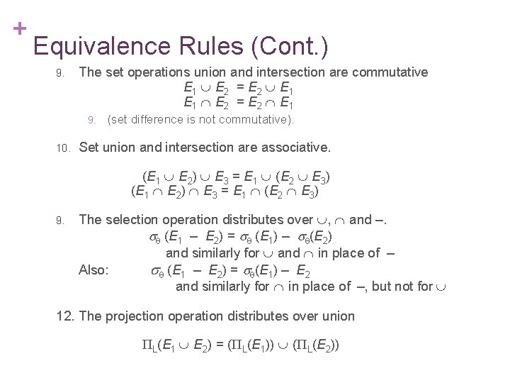
+ Equivalence Rules (Cont. ) 9. The set operations union and intersection are commutative E 1 E 2 = E 2 E 1 9. 10. (set difference is not commutative). Set union and intersection are associative. (E 1 E 2) E 3 = E 1 (E 2 E 3) 9. The selection operation distributes over , and –. (E 1 – E 2) = (E 1) – (E 2) and similarly for and in place of – Also: (E 1 – E 2) = (E 1) – E 2 and similarly for in place of –, but not for 12. The projection operation distributes over union L(E 1 E 2) = ( L(E 1)) ( L(E 2))

+ Housekeeping (Apr 3) n Assignment n Project 4 marking requirements and QA

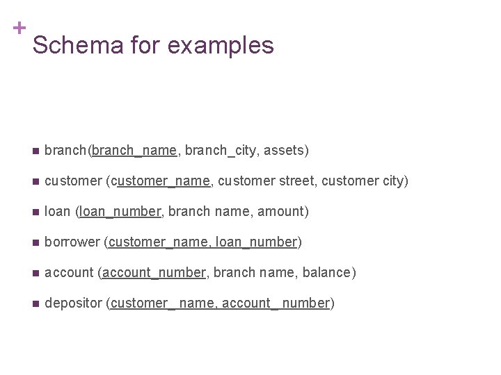
+ Schema for examples n branch(branch_name, branch_city, assets) n customer (customer_name, customer street, customer city) n loan (loan_number, branch name, amount) n borrower (customer_name, loan_number) n account (account_number, branch name, balance) n depositor (customer_ name, account_ number)

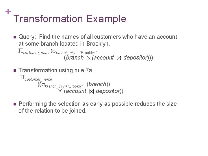
+ Transformation Example n Query: Find the names of all customers who have an account at some branch located in Brooklyn. customer_name( branch_city = “Brooklyn” (branch (account depositor))) n Transformation using rule 7 a. customer_name (( branch_city =“Brooklyn” (branch)) (account depositor)) n Performing the selection as early as possible reduces the size of the relation to be joined.

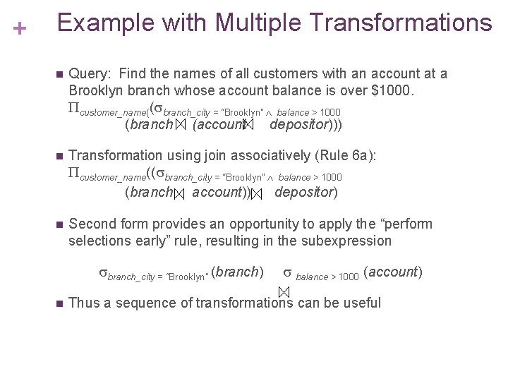
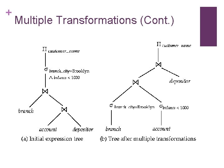
+ Example with Multiple Transformations n Query: Find the names of all customers with an account at a Brooklyn branch whose account balance is over $1000. customer_name(( branch_city = “Brooklyn” balance > 1000 (branch (account depositor))) n Transformation using join associatively (Rule 6 a): customer_name(( branch_city = “Brooklyn” balance > 1000 (branch account)) depositor) n Second form provides an opportunity to apply the “perform selections early” rule, resulting in the subexpression branch_city = “Brooklyn” (branch) n balance > 1000 (account) Thus a sequence of transformations can be useful

+ Multiple Transformations (Cont. )

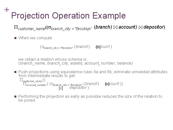
+ Projection Operation Example customer_name(( branch_city = “Brooklyn” (branch) n account) depositor) When we compute ( branch_city = “Brooklyn” (branch) account ) we obtain a relation whose schema is: (branch_name, branch_city, assets, account_number, balance) n Push projections using equivalence rules 8 a and 8 b; eliminate unneeded attributes from intermediate results to get: customer_name (( account_number ( ( branch_city = “Brooklyn” (branch) account )) depositor ) n Performing the projection as early as possible reduces the size of the relation to be joined.

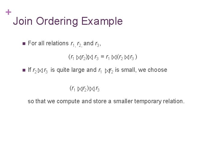
+ Join Ordering Example n For all relations r 1, r 2, and r 3, (r 1 n If r 2 ) r 3 = r 1 r 3 is quite large and r 1 (r 1 r 2 ) (r 2 r 3 ) r 2 is small, we choose r 3 so that we compute and store a smaller temporary relation.

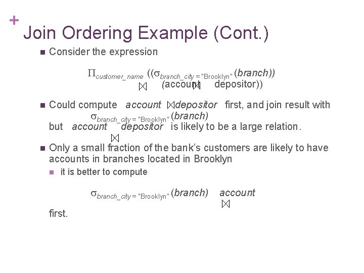
+ Join Ordering Example (Cont. ) n Consider the expression customer_name (( branch_city = “Brooklyn” (branch)) (account depositor)) n Could compute account depositor first, and join result with branch_city = “Brooklyn” (branch) but account depositor is likely to be a large relation. n Only a small fraction of the bank’s customers are likely to have accounts in branches located in Brooklyn n it is better to compute branch_city = “Brooklyn” (branch) first. account

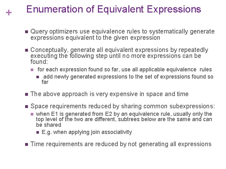
+ Enumeration of Equivalent Expressions n Query optimizers use equivalence rules to systematically generate expressions equivalent to the given expression n Conceptually, generate all equivalent expressions by repeatedly executing the following step until no more expressions can be found: n for each expression found so far, use all applicable equivalence rules n add newly generated expressions to the set of expressions found so far n The above approach is very expensive in space and time n Space requirements reduced by sharing common subexpressions: n n when E 1 is generated from E 2 by an equivalence rule, usually only the top level of the two are different, subtrees below are the same and can be shared n E. g. when applying join associativity Time requirements are reduced by not generating all expressions

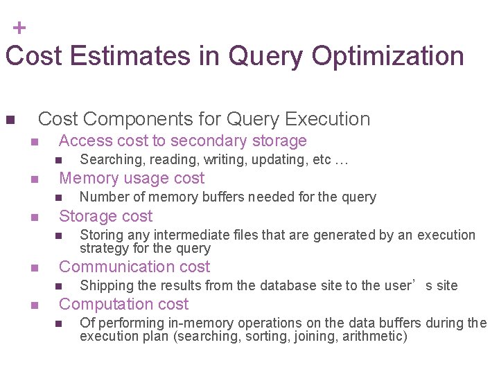
+ Cost Estimates in Query Optimization n Cost Components for Query Execution n Access cost to secondary storage n n Memory usage cost n n Storing any intermediate files that are generated by an execution strategy for the query Communication cost n n Number of memory buffers needed for the query Storage cost n n Searching, reading, writing, updating, etc … Shipping the results from the database site to the user’s site Computation cost n Of performing in-memory operations on the data buffers during the execution plan (searching, sorting, joining, arithmetic)

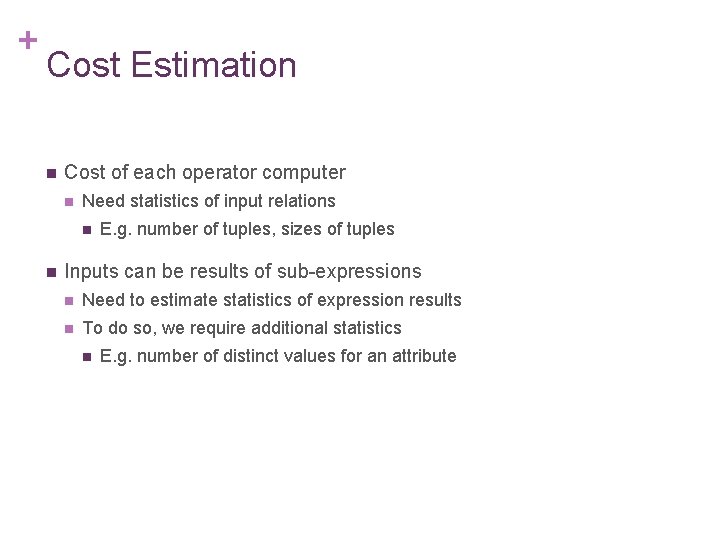
+ Cost Estimation n Cost of each operator computer n Need statistics of input relations n n E. g. number of tuples, sizes of tuples Inputs can be results of sub-expressions n Need to estimate statistics of expression results n To do so, we require additional statistics n E. g. number of distinct values for an attribute

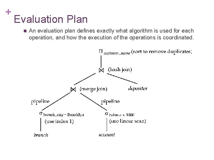
+ Evaluation Plan n An evaluation plan defines exactly what algorithm is used for each operation, and how the execution of the operations is coordinated.

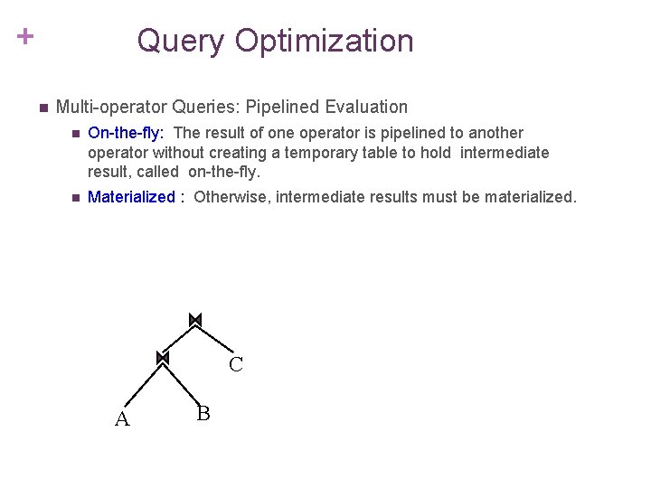
+ Query Optimization n Multi-operator Queries: Pipelined Evaluation n On-the-fly: The result of one operator is pipelined to another operator without creating a temporary table to hold intermediate result, called on-the-fly. n Materialized : Otherwise, intermediate results must be materialized. C A B

+ Choice of Evaluation Plans n n Must consider the interaction of evaluation techniques when choosing evaluation plans: choosing the cheapest algorithm for each operation independently may not yield best overall algorithm. E. g. n merge-join may be costlier than hash-join, but may provide a sorted output which reduces the cost for an outer level aggregation. n nested-loop join may provide opportunity for pipelining Practical query optimizers incorporate elements of the following two broad approaches: 1. Search all the plans and choose the best plan in a cost-based fashion. (slides at back of deck if interested) 2. Uses heuristics to choose a plan.

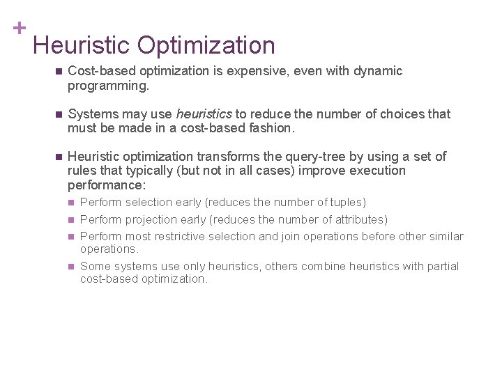
+ Heuristic Optimization n Cost-based optimization is expensive, even with dynamic programming. n Systems may use heuristics to reduce the number of choices that must be made in a cost-based fashion. n Heuristic optimization transforms the query-tree by using a set of rules that typically (but not in all cases) improve execution performance: n n Perform selection early (reduces the number of tuples) Perform projection early (reduces the number of attributes) Perform most restrictive selection and join operations before other similar operations. Some systems use only heuristics, others combine heuristics with partial cost-based optimization.

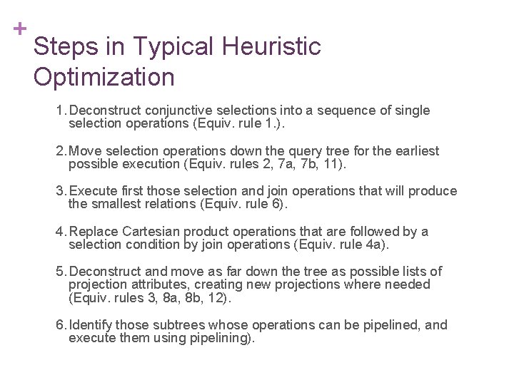
+ Steps in Typical Heuristic Optimization 1. Deconstruct conjunctive selections into a sequence of single selection operations (Equiv. rule 1. ). 2. Move selection operations down the query tree for the earliest possible execution (Equiv. rules 2, 7 a, 7 b, 11). 3. Execute first those selection and join operations that will produce the smallest relations (Equiv. rule 6). 4. Replace Cartesian product operations that are followed by a selection condition by join operations (Equiv. rule 4 a). 5. Deconstruct and move as far down the tree as possible lists of projection attributes, creating new projections where needed (Equiv. rules 3, 8 a, 8 b, 12). 6. Identify those subtrees whose operations can be pipelined, and execute them using pipelining).

+ Additional slides Structure of Query Optimizers More details about cost estimation

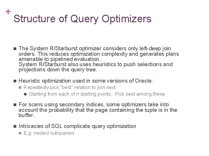
+ Structure of Query Optimizers n The System R/Starburst optimizer considers only left-deep join orders. This reduces optimization complexity and generates plans amenable to pipelined evaluation. System R/Starburst also uses heuristics to push selections and projections down the query tree. n Heuristic optimization used in some versions of Oracle: n Repeatedly pick “best” relation to join next n Starting from each of n starting points. Pick best among these. n For scans using secondary indices, some optimizers take into account the probability that the page containing the tuple is in the buffer. n Intricacies of SQL complicate query optimization n E. g. nested subqueries

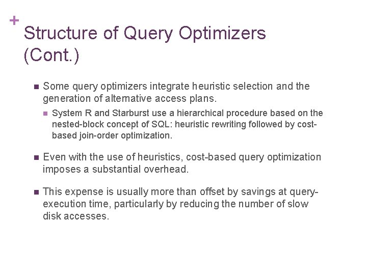
+ Structure of Query Optimizers (Cont. ) n Some query optimizers integrate heuristic selection and the generation of alternative access plans. n System R and Starburst use a hierarchical procedure based on the nested-block concept of SQL: heuristic rewriting followed by costbased join-order optimization. n Even with the use of heuristics, cost-based query optimization imposes a substantial overhead. n This expense is usually more than offset by savings at queryexecution time, particularly by reducing the number of slow disk accesses.

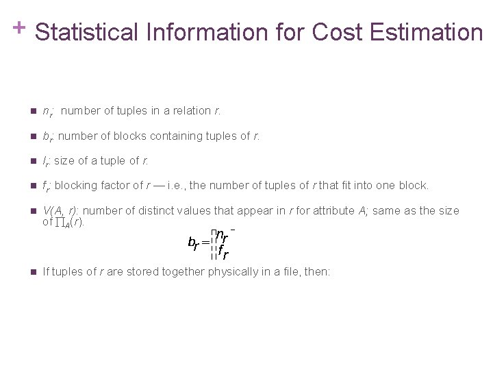
+ Statistical Information for Cost Estimation n nr: number of tuples in a relation r. n br: number of blocks containing tuples of r. n lr : size of a tuple of r. n fr: blocking factor of r — i. e. , the number of tuples of r that fit into one block. n V(A, r): number of distinct values that appear in r for attribute A; same as the size of A(r). n If tuples of r are stored together physically in a file, then:

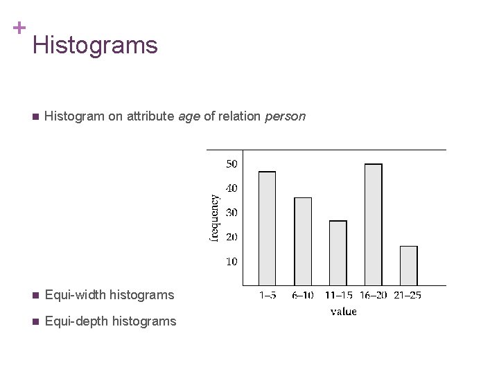
+ Histograms n Histogram on attribute age of relation person n Equi-width histograms n Equi-depth histograms

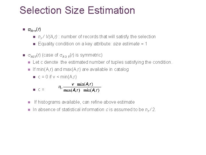
Selection Size Estimation n n A=v(r) n nr / V(A, r) : number of records that will satisfy the selection n Equality condition on a key attribute: size estimate = 1 A V(r) (case of A V(r) is symmetric) n Let c denote the estimated number of tuples satisfying the condition. n If min(A, r) and max(A, r) are available in catalog n n n c = 0 if v < min(A, r) n c= If histograms available, can refine above estimate In absence of statistical information c is assumed to be nr / 2.

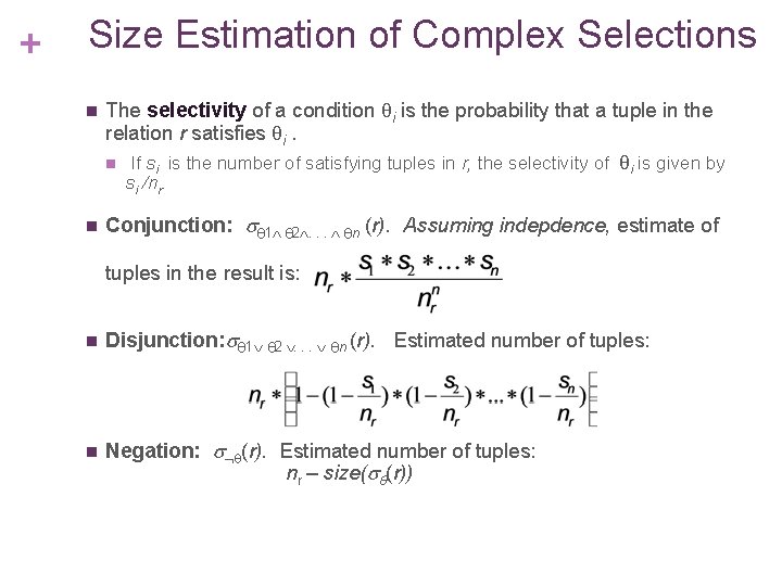
+ Size Estimation of Complex Selections n The selectivity of a condition i is the probability that a tuple in the relation r satisfies i. n If si is the number of satisfying tuples in r, the selectivity of i is given by si /nr. n Conjunction: 1 2. . . n (r). Assuming indepdence, estimate of tuples in the result is: n Disjunction: 1 2 . . . n (r). Estimated number of tuples: n Negation: (r). Estimated number of tuples: nr – size( (r))

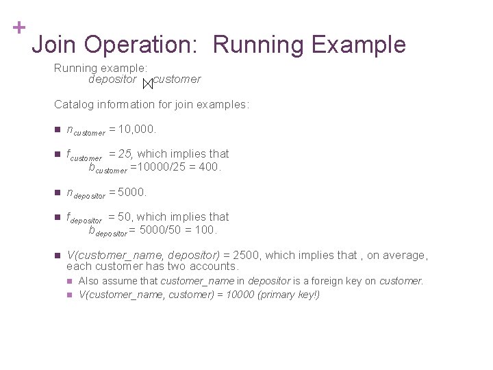
+ Join Operation: Running Example Running example: depositor customer Catalog information for join examples: n ncustomer = 10, 000. n fcustomer = 25, which implies that bcustomer =10000/25 = 400. n ndepositor = 5000. n fdepositor = 50, which implies that bdepositor = 5000/50 = 100. n V(customer_name, depositor) = 2500, which implies that , on average, each customer has two accounts. n n Also assume that customer_name in depositor is a foreign key on customer. V(customer_name, customer) = 10000 (primary key!)

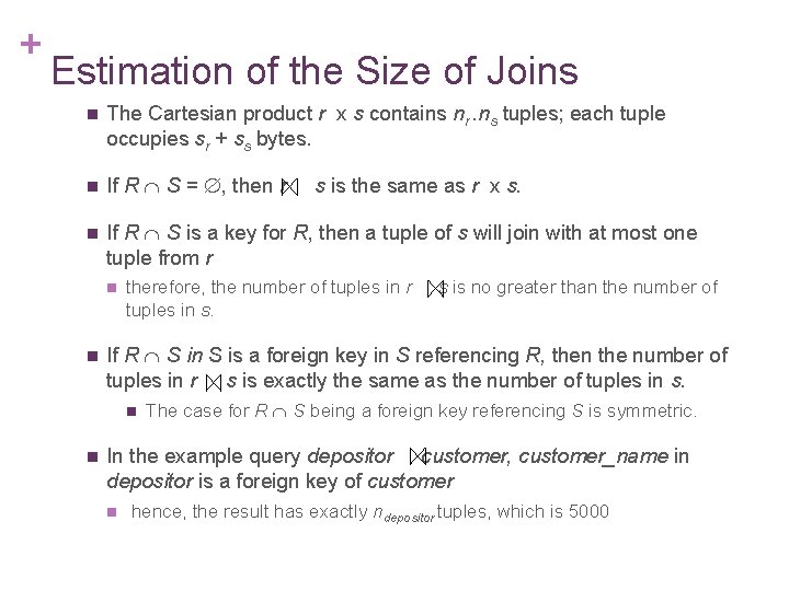
+ Estimation of the Size of Joins n The Cartesian product r x s contains nr. ns tuples; each tuple occupies sr + ss bytes. n If R S = , then r n If R S is a key for R, then a tuple of s will join with at most one tuple from r n n therefore, the number of tuples in r tuples in s. s is no greater than the number of If R S in S is a foreign key in S referencing R, then the number of tuples in r s is exactly the same as the number of tuples in s. n n s is the same as r x s. The case for R S being a foreign key referencing S is symmetric. In the example query depositor customer, customer_name in depositor is a foreign key of customer n hence, the result has exactly ndepositor tuples, which is 5000

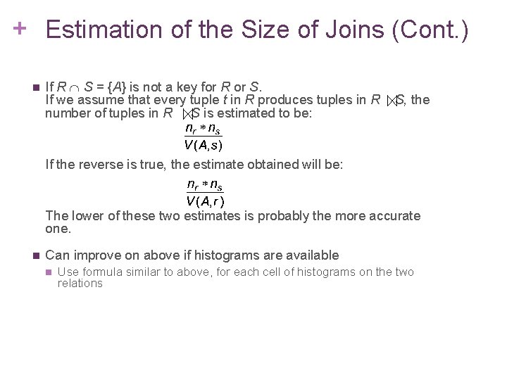
+ Estimation of the Size of Joins (Cont. ) n If R S = {A} is not a key for R or S. If we assume that every tuple t in R produces tuples in R number of tuples in R S is estimated to be: S, the If the reverse is true, the estimate obtained will be: The lower of these two estimates is probably the more accurate one. n Can improve on above if histograms are available n Use formula similar to above, for each cell of histograms on the two relations

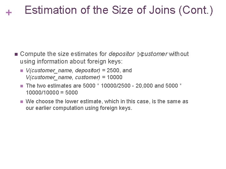
Estimation of the Size of Joins (Cont. ) + n Compute the size estimates for depositor using information about foreign keys: customer without n V(customer_name, depositor) = 2500, and V(customer_name, customer) = 10000 n The two estimates are 5000 * 10000/2500 - 20, 000 and 5000 * 10000/10000 = 5000 n We choose the lower estimate, which in this case, is the same as our earlier computation using foreign keys.

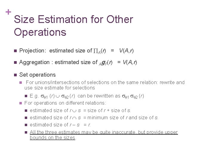
+ Size Estimation for Other Operations n Projection: estimated size of A(r) = V(A, r) n Aggregation : estimated size of Ag. F(r) = V(A, r) n Set operations n For unions/intersections of selections on the same relation: rewrite and use size estimate for selections E. g. 1 (r) 2 (r) can be rewritten as 1 2 (r) For operations on different relations: n estimated size of r s = size of r + size of s. n estimated size of r s = minimum size of r and size of s. n estimated size of r – s = r. n All the three estimates may be quite inaccurate, but provide upper bounds on the sizes. n n

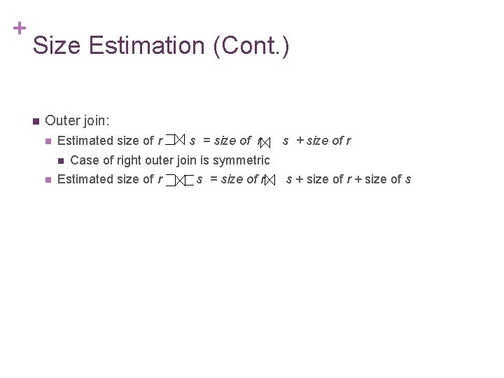
+ Size Estimation (Cont. ) n Outer join: n Estimated size of r n n s = size of r s + size of r Case of right outer join is symmetric Estimated size of r s = size of r s + size of r + size of s

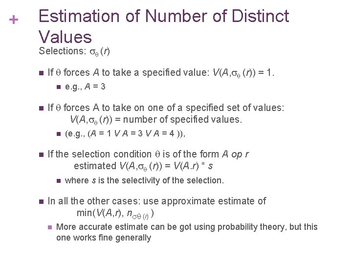
+ Estimation of Number of Distinct Values Selections: (r) n If forces A to take a specified value: V(A, (r)) = 1. n n If forces A to take on one of a specified set of values: V(A, (r)) = number of specified values. n n (e. g. , (A = 1 V A = 3 V A = 4 )), If the selection condition is of the form A op r estimated V(A, (r)) = V(A. r) * s n n e. g. , A = 3 where s is the selectivity of the selection. In all the other cases: use approximate estimate of min(V(A, r), n (r) ) n More accurate estimate can be got using probability theory, but this one works fine generally

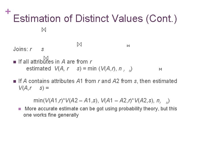
+ Estimation of Distinct Values (Cont. ) Joins: r n n s If all attributes in A are from r estimated V(A, r s) = min (V(A, r), n r s) If A contains attributes A 1 from r and A 2 from s, then estimated V(A, r s) = min(V(A 1, r)*V(A 2 – A 1, s), V(A 1 – A 2, r)*V(A 2, s), nr n s) More accurate estimate can be got using probability theory, but this one works fine generally

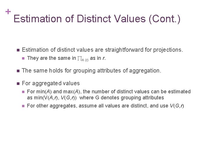
+ Estimation of Distinct Values (Cont. ) n Estimation of distinct values are straightforward for projections. n They are the same in A (r) as in r. n The same holds for grouping attributes of aggregation. n For aggregated values n For min(A) and max(A), the number of distinct values can be estimated as min(V(A, r), V(G, r)) where G denotes grouping attributes n For other aggregates, assume all values are distinct, and use V(G, r)

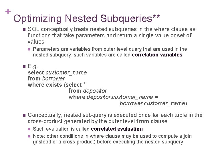
+ Optimizing Nested Subqueries** n SQL conceptually treats nested subqueries in the where clause as functions that take parameters and return a single value or set of values n Parameters are variables from outer level query that are used in the nested subquery; such variables are called correlation variables n E. g. select customer_name from borrower where exists (select * from depositor where depositor. customer_name = borrower. customer_name) n Conceptually, nested subquery is executed once for each tuple in the cross-product generated by the outer level from clause n n Such evaluation is called correlated evaluation Note: other conditions in where clause may be used to compute a join (instead of a cross-product) before executing the nested subquery

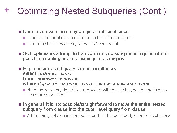
+ Optimizing Nested Subqueries (Cont. ) n Correlated evaluation may be quite inefficient since n n a large number of calls may be made to the nested query there may be unnecessary random I/O as a result n SQL optimizers attempt to transform nested subqueries to joins where possible, enabling use of efficient join techniques n E. g. : earlier nested query can be rewritten as select customer_name from borrower, depositor where depositor. customer_name = borrower. customer_name n n Note: above query doesn’t correctly deal with duplicates, can be modified to do so as we will see In general, it is not possible/straightforward to move the entire nested subquery from clause into the outer level query from clause n A temporary relation is created instead, and used in body of outer level query

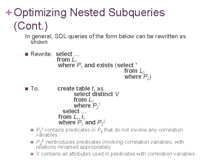
+ Optimizing Nested Subqueries (Cont. ) In general, SQL queries of the form below can be rewritten as shown n Rewrite: select … from L 1 where P 1 and exists (select * from L 2 where P 2) n To: n n n create table t 1 as select distinct V from L 2 where P 21 select … from L 1, t 1 where P 1 and P 22 P 21 contains predicates in P 2 that do not involve any correlation variables P 22 reintroduces predicates involving correlation variables, with relations renamed appropriately V contains all attributes used in predicates with correlation variables

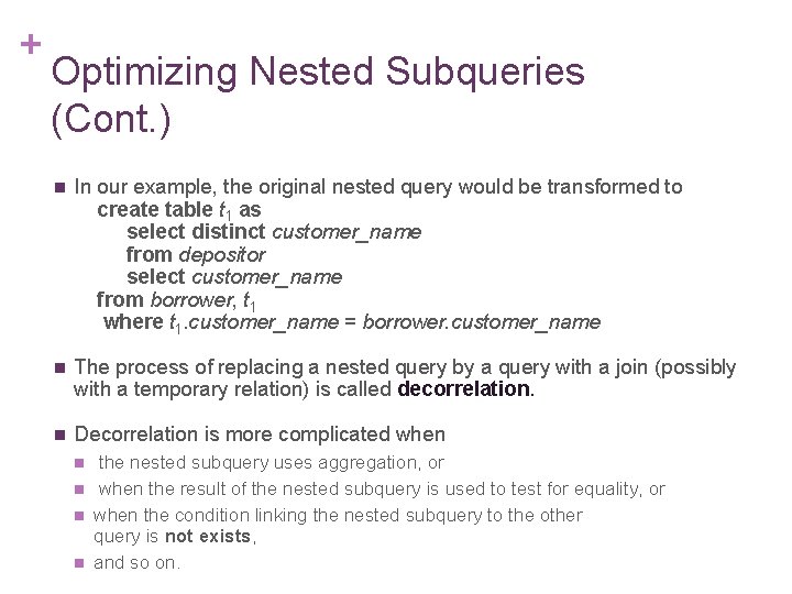
+ Optimizing Nested Subqueries (Cont. ) n In our example, the original nested query would be transformed to create table t 1 as select distinct customer_name from depositor select customer_name from borrower, t 1 where t 1. customer_name = borrower. customer_name n The process of replacing a nested query by a query with a join (possibly with a temporary relation) is called decorrelation. n Decorrelation is more complicated when n n the nested subquery uses aggregation, or when the result of the nested subquery is used to test for equality, or when the condition linking the nested subquery to the other query is not exists, and so on.

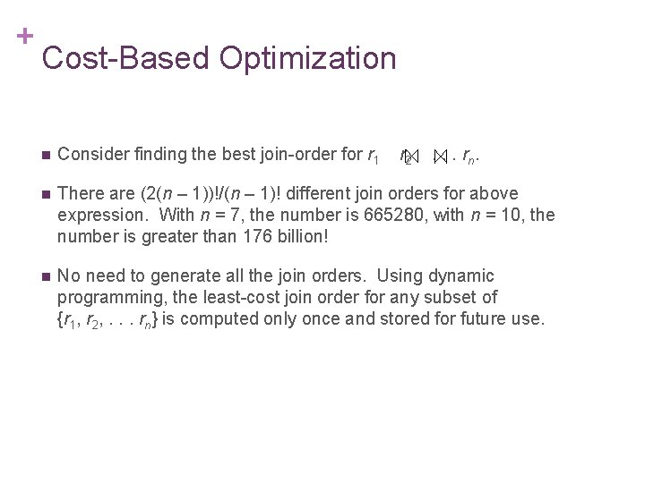
+ Cost-Based Optimization n Consider finding the best join-order for r 1 r 2 . . . rn. n There are (2(n – 1))!/(n – 1)! different join orders for above expression. With n = 7, the number is 665280, with n = 10, the number is greater than 176 billion! n No need to generate all the join orders. Using dynamic programming, the least-cost join order for any subset of {r 1, r 2, . . . rn} is computed only once and stored for future use.

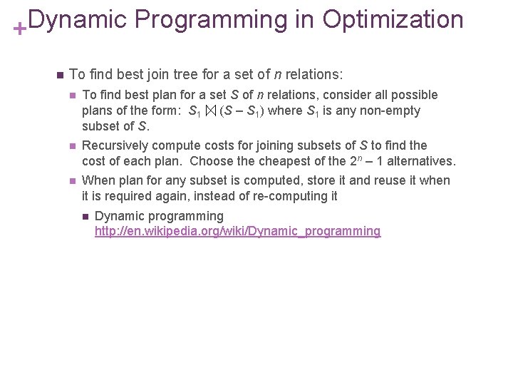
Dynamic Programming in Optimization + n To find best join tree for a set of n relations: n To find best plan for a set S of n relations, consider all possible plans of the form: S 1 (S – S 1) where S 1 is any non-empty subset of S. n Recursively compute costs for joining subsets of S to find the cost of each plan. Choose the cheapest of the 2 n – 1 alternatives. n When plan for any subset is computed, store it and reuse it when it is required again, instead of re-computing it n Dynamic programming http: //en. wikipedia. org/wiki/Dynamic_programming

+ Join Order Optimization Algorithm procedure findbestplan(S) if (bestplan[S]. cost ) return bestplan[S] // else bestplan[S] has not been computed earlier, compute it now if (S contains only 1 relation) set bestplan[S]. plan and bestplan[S]. cost based on the best way of accessing S else for each non-empty subset S 1 of S such that S 1 S P 1= findbestplan(S 1) P 2= findbestplan(S - S 1) A = best algorithm for joining results of P 1 and P 2 cost = P 1. cost + P 2. cost + cost of A if cost < bestplan[S]. cost = cost bestplan[S]. plan = “execute P 1. plan; execute P 2. plan; join results of P 1 and P 2 using A” return bestplan[S]

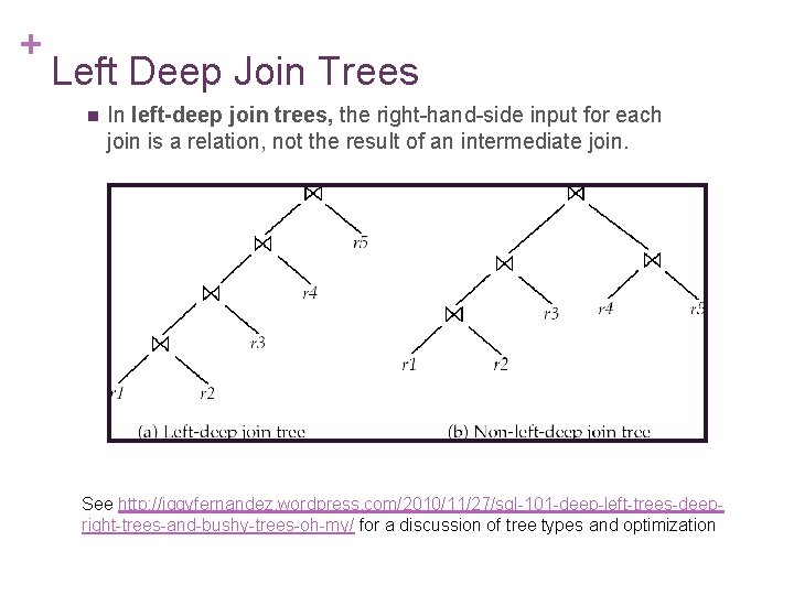
+ Left Deep Join Trees n In left-deep join trees, the right-hand-side input for each join is a relation, not the result of an intermediate join. See http: //iggyfernandez. wordpress. com/2010/11/27/sql-101 -deep-left-trees-deepright-trees-and-bushy-trees-oh-my/ for a discussion of tree types and optimization

+ Cost of Optimization n With dynamic programming, time complexity of optimization with bushy trees is O(3 n). (see http: //en. wikipedia. org/wiki/Big_O_notation) n n n Space complexity is O(2 n) n n n Consider n alternatives with one relation as right-hand side input and the other relations as left-hand side input. Using (recursively computed and stored) least-cost join order for each alternative on left-hand-side, choose the cheapest of the n alternatives. If only left-deep trees are considered, time complexity of finding best join order is O(n 2 n) n n space complexity = amount of memory an algorithm needs To find best left-deep join tree for a set of n relations: n n With n = 10, this number is 59000 instead of 176 billion! time complexity of an algorithm quantifies the amount of time taken by an algorithm to run as a function of the length of the string representing the input Space complexity remains at O(2 n) Cost-based optimization is expensive, but worthwhile for queries on large datasets (typical queries have small n, generally < 10)

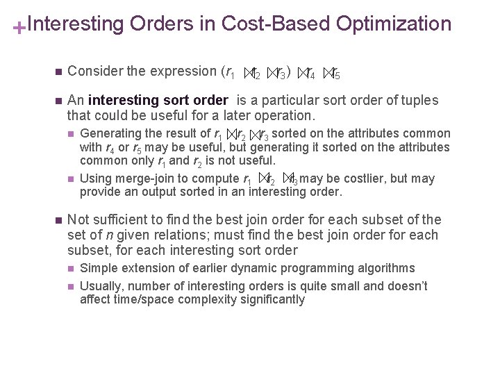
+Interesting Orders in Cost-Based Optimization n Consider the expression (r 1 n An interesting sort order is a particular sort order of tuples that could be useful for a later operation. n n n r 2 r 3 ) r 4 r 5 Generating the result of r 1 r 2 r 3 sorted on the attributes common with r 4 or r 5 may be useful, but generating it sorted on the attributes common only r 1 and r 2 is not useful. Using merge-join to compute r 1 r 2 r 3 may be costlier, but may provide an output sorted in an interesting order. Not sufficient to find the best join order for each subset of the set of n given relations; must find the best join order for each subset, for each interesting sort order n n Simple extension of earlier dynamic programming algorithms Usually, number of interesting orders is quite small and doesn’t affect time/space complexity significantly