Unconstrained Optimization Rong Jin Recap o Gradient ascentdescent

Unconstrained Optimization Rong Jin

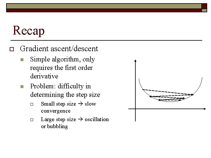
Recap o Gradient ascent/descent n n Simple algorithm, only requires the first order derivative Problem: difficulty in determining the step size o o Small step size slow convergence Large step size oscillation or bubbling

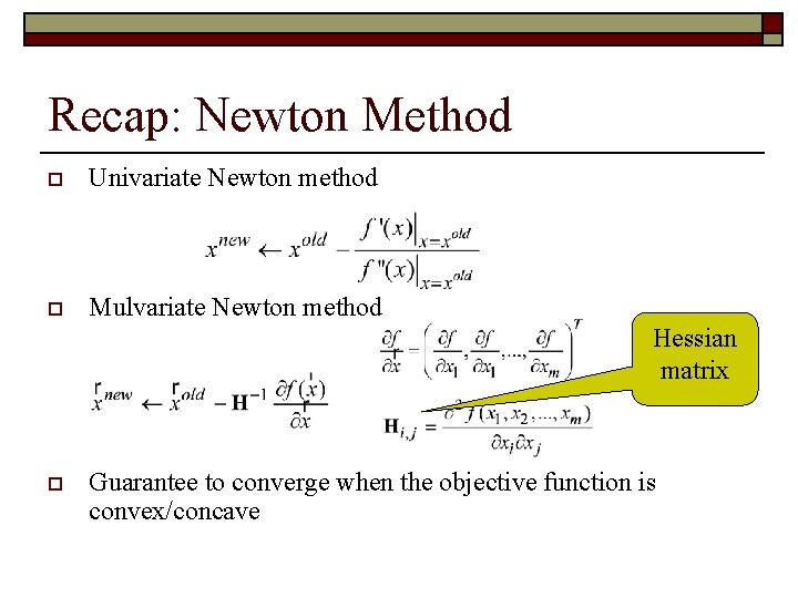
Recap: Newton Method o Univariate Newton method o Mulvariate Newton method Hessian matrix o Guarantee to converge when the objective function is convex/concave

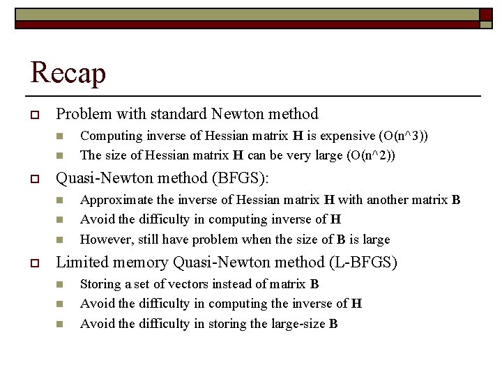
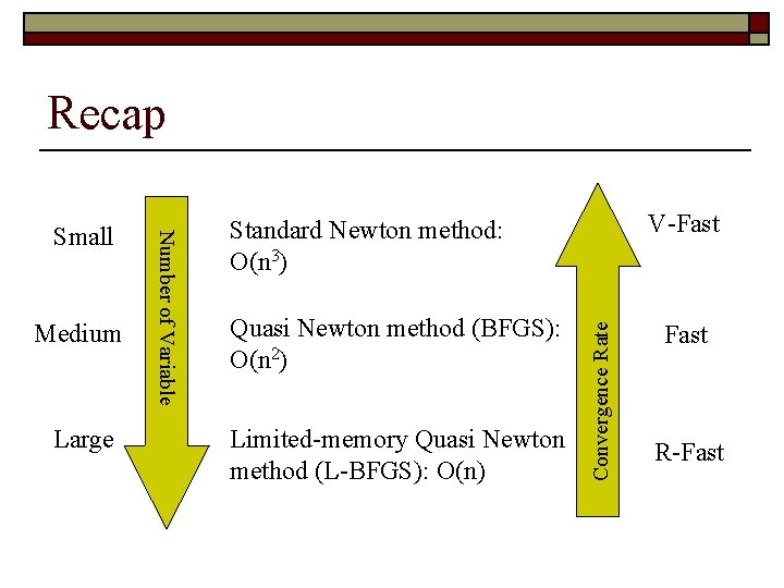
Recap o Problem with standard Newton method n n o Quasi-Newton method (BFGS): n n n o Computing inverse of Hessian matrix H is expensive (O(n^3)) The size of Hessian matrix H can be very large (O(n^2)) Approximate the inverse of Hessian matrix H with another matrix B Avoid the difficulty in computing inverse of H However, still have problem when the size of B is large Limited memory Quasi-Newton method (L-BFGS) n n n Storing a set of vectors instead of matrix B Avoid the difficulty in computing the inverse of H Avoid the difficulty in storing the large-size B

Recap Large V-Fast Standard Newton method: O(n 3) Quasi Newton method (BFGS): O(n 2) Limited-memory Quasi Newton method (L-BFGS): O(n) Convergence Rate Medium Number of Variable Small Fast R-Fast

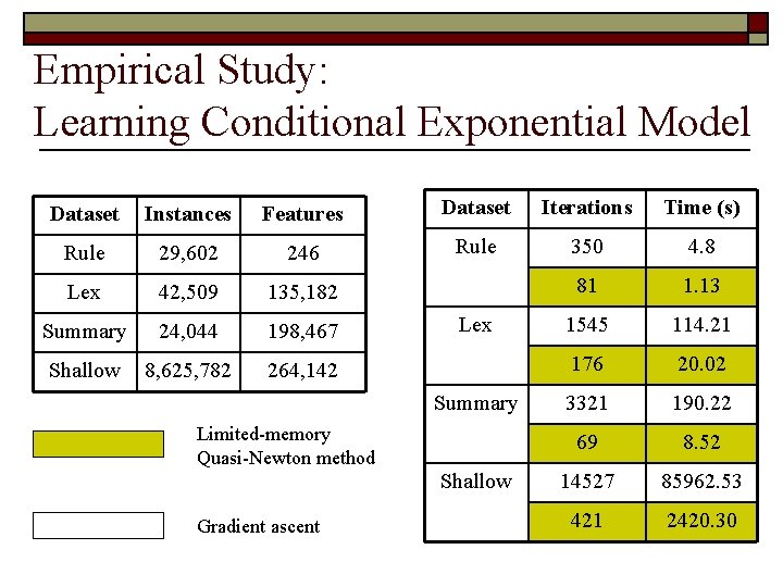
Empirical Study: Learning Conditional Exponential Model Dataset Instances Features Dataset Iterations Time (s) Rule 29, 602 246 Rule 350 4. 8 Lex 42, 509 135, 182 81 1. 13 Summary 24, 044 198, 467 1545 114. 21 Shallow 8, 625, 782 264, 142 176 20. 02 3321 190. 22 69 8. 52 14527 85962. 53 421 2420. 30 Lex Summary Limited-memory Quasi-Newton method Shallow Gradient ascent

Free Software o http: //www. ece. northwestern. edu/~nocedal/so ftware. html n n L-BFGSB

Conjugate Gradient o Another Great Numerical Optimization Method !

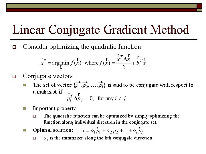
Linear Conjugate Gradient Method o Consider optimizing the quadratic function o Conjugate vectors n The set of vector {p 1, p 2, …, pl} is said to be conjugate with respect to a matrix A if n Important property o n The quadratic function can be optimized by simply optimizing the function along individual direction in the conjugate set. Optimal solution: o k is the minimizer along the kth conjugate direction

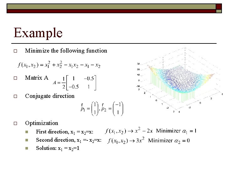
Example o Minimize the following function o Matrix A o Conjugate direction o Optimization n First direction, x 1 = x 2=x: Second direction, x 1 =- x 2=x: Solution: x 1 = x 2=1

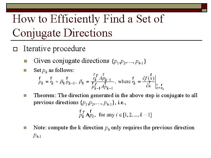
How to Efficiently Find a Set of Conjugate Directions o Iterative procedure n Given conjugate directions {p 1, p 2, …, pk-1} n Set pk as follows: n Theorem: The direction generated in the above step is conjugate to all previous directions {p 1, p 2, …, pk-1}, i. e. , n Note: compute the k direction pk only requires the previous direction pk-1

Nonlinear Conjugate Gradient o Even though conjugate gradient is derived for a quadratic objective function, it can be applied directly to other nonlinear functions n o Guarantee convergence if the objective is convex/concave Variants: n n Fletcher-Reeves conjugate gradient (FR-CG) Polak-Ribiere conjugate gradient (PR-CG) o o More robust than FR-CG Compared to Newton method n n n The first order method Usually less efficient than Newton method However, it is simple to implement

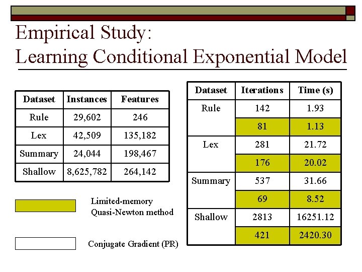
Empirical Study: Learning Conditional Exponential Model Dataset Instances Features Rule 29, 602 246 Lex 42, 509 135, 182 Summary 24, 044 198, 467 Shallow 8, 625, 782 264, 142 Limited-memory Quasi-Newton method Conjugate Gradient (PR) Dataset Iterations Time (s) Rule 142 1. 93 81 1. 13 281 21. 72 176 20. 02 537 31. 66 69 8. 52 2813 16251. 12 421 2420. 30 Lex Summary Shallow

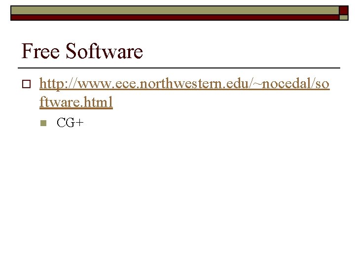
Free Software o http: //www. ece. northwestern. edu/~nocedal/so ftware. html n CG+

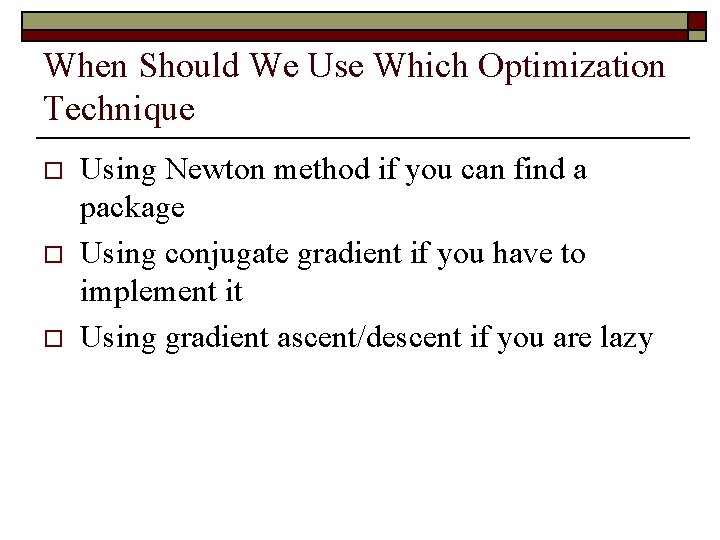
When Should We Use Which Optimization Technique o o o Using Newton method if you can find a package Using conjugate gradient if you have to implement it Using gradient ascent/descent if you are lazy

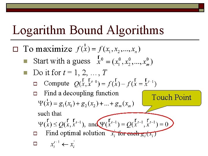
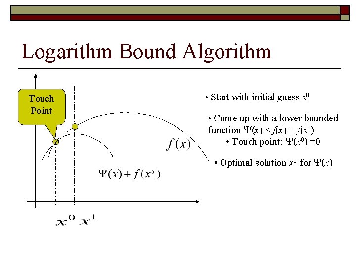
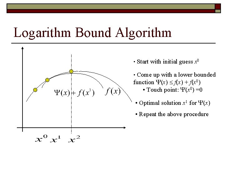
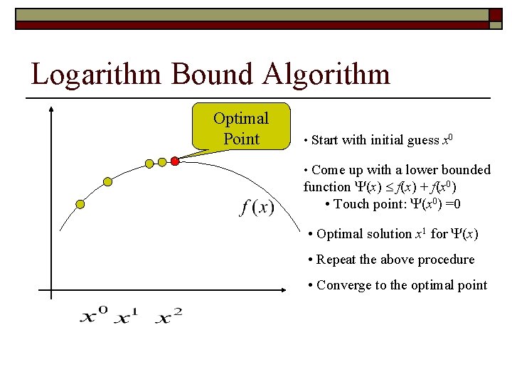
Logarithm Bound Algorithms o To maximize n n Start with a guess Do it for t = 1, 2, …, T o o Compute Find a decoupling function Find optimal solution Touch Point

Logarithm Bound Algorithm Touch Point • Start with initial guess x 0 • Come up with a lower bounded function (x) f(x) + f(x 0) • Touch point: (x 0) =0 • Optimal solution x 1 for (x)

Logarithm Bound Algorithm • Start with initial guess x 0 • Come up with a lower bounded function (x) f(x) + f(x 0) • Touch point: (x 0) =0 • Optimal solution x 1 for (x) • Repeat the above procedure

Logarithm Bound Algorithm Optimal Point • Start with initial guess x 0 • Come up with a lower bounded function (x) f(x) + f(x 0) • Touch point: (x 0) =0 • Optimal solution x 1 for (x) • Repeat the above procedure • Converge to the optimal point

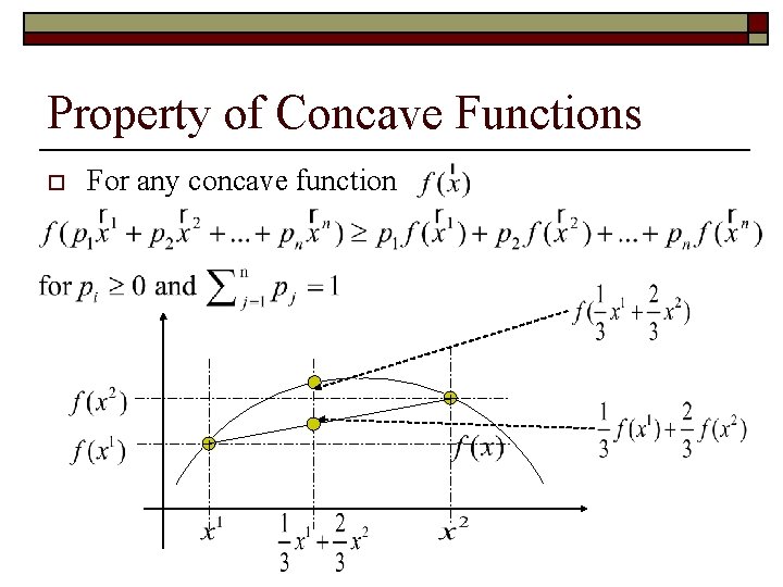
Property of Concave Functions o For any concave function

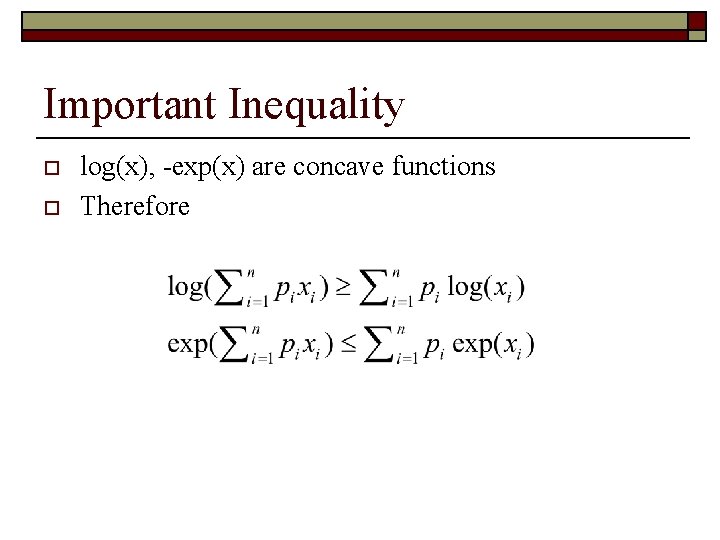
Important Inequality o o log(x), -exp(x) are concave functions Therefore

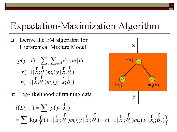
Expectation-Maximization Algorithm o Derive the EM algorithm for Hierarchical Mixture Model X r(x) m 1(x) o Log-likelihood of training data m 2(x) y