Unconditional Weak derandomization of weak algorithms Explicit versions

Unconditional Weak derandomization of weak algorithms : Explicit versions of Yao’s lemma Ronen Shaltiel, University of Haifa

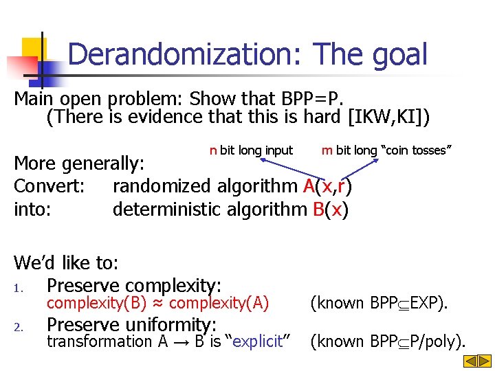
Derandomization: The goal Main open problem: Show that BPP=P. (There is evidence that this is hard [IKW, KI]) n bit long input m bit long “coin tosses” More generally: Convert: randomized algorithm A(x, r) into: deterministic algorithm B(x) We’d like to: 1. Preserve complexity: complexity(B) ≈ complexity(A) 2. Preserve uniformity: transformation A → B is “explicit” (known BPP EXP). (known BPP P/poly).

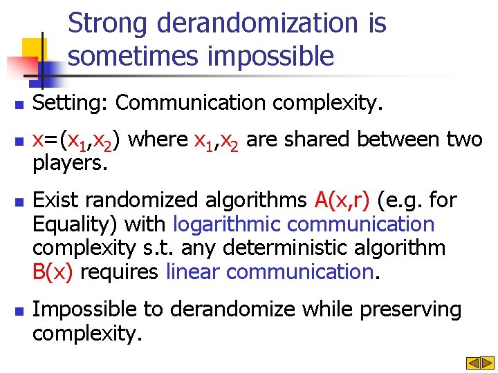
Strong derandomization is sometimes impossible n n Setting: Communication complexity. x=(x 1, x 2) where x 1, x 2 are shared between two players. Exist randomized algorithms A(x, r) (e. g. for Equality) with logarithmic communication complexity s. t. any deterministic algorithm B(x) requires linear communication. Impossible to derandomize while preserving complexity.

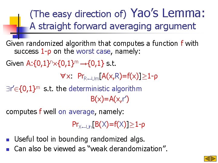
(The easy direction of) Yao’s Lemma: A straight forward averaging argument Given randomized algorithm that computes a function f with success 1 -ρ on the worst case, namely: Given A: {0, 1}n£{0, 1}m →{0, 1} s. t. ∀x: Pr. R←Um[A(x, R)=f(x)]¸ 1 -ρ r’ 2{0, 1}m s. t. the deterministic algorithm B(x)=A(x, r’) computes f well on average, namely: Pr. X←Un[B(X)=f(X)]¸ 1 -ρ n n Useful tool in bounding randomized algs. Can also be viewed as “weak derandomization”.

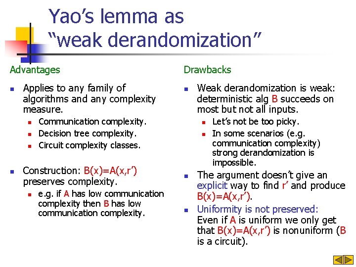
Yao’s lemma as “weak derandomization” Advantages n Applies to any family of algorithms and any complexity measure. n n n Communication complexity. Decision tree complexity. Circuit complexity classes. Construction: B(x)=A(x, r’) preserves complexity. n Drawbacks e. g. if A has low communication complexity then B has low communication complexity. Weak derandomization is weak: deterministic alg B succeeds on most but not all inputs. n n Let’s not be too picky. In some scenarios (e. g. communication complexity) strong derandomization is impossible. The argument doesn’t give an explicit way to find r’ and produce B(x)=A(x, r’). Uniformity is not preserved: Even if A is uniform we only get that B(x)=A(x, r’) is nonuniform (B is a circuit).

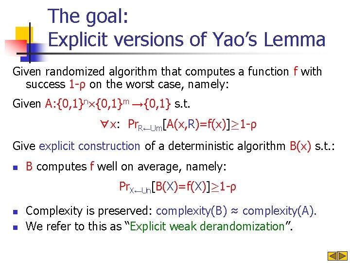
The goal: Explicit versions of Yao’s Lemma Given randomized algorithm that computes a function f with success 1 -ρ on the worst case, namely: Given A: {0, 1}n£{0, 1}m →{0, 1} s. t. ∀x: Pr. R←Um[A(x, R)=f(x)]¸ 1 -ρ Give explicit construction of a deterministic algorithm B(x) s. t. : n B computes f well on average, namely: Pr. X←Un[B(X)=f(X)]¸ 1 -ρ n n Complexity is preserved: complexity(B) ≈ complexity(A). We refer to this as “Explicit weak derandomization”.

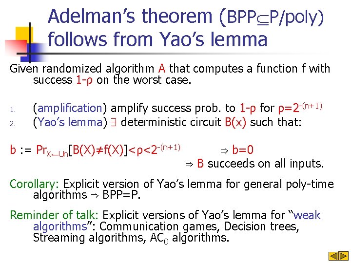
Adelman’s theorem (BPP P/poly) follows from Yao’s lemma Given randomized algorithm A that computes a function f with success 1 -ρ on the worst case. 1. 2. (amplification) amplify success prob. to 1 -ρ for ρ=2 -(n+1) (Yao’s lemma) deterministic circuit B(x) such that: b : = Pr. X←Un[B(X)≠f(X)]<ρ<2 -(n+1) ⇒ b=0 ⇒ B succeeds on all inputs. Corollary: Explicit version of Yao’s lemma for general poly-time algorithms ⇒ BPP=P. Reminder of talk: Explicit versions of Yao’s lemma for “weak algorithms”: Communication games, Decision trees, Streaming algorithms, AC 0 algorithms.

Related work: Extracting randomness from the input Idea [Goldreich and Wigderson]: Given a randomized alg A(x, r) s. t. |r|·|x| consider the deterministic alg: B(x)=A(x, x). Intuition: If input x is chosen at random then random coins r: =x is chosen at random. Problem: Input and coins are correlated. consider A s. t. 8 input x, coin x is bad for x). (e. g. GW: Does work if A has the additional property that whether or not a coin toss is good does not depend on the input. GW: It turns out that there are A’s with this property.

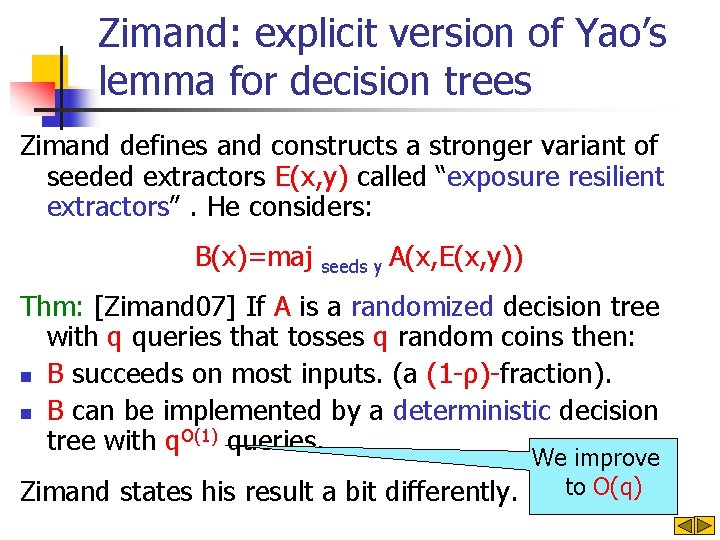
The role of extractors in [GW] In their paper Goldreich and Wigderson actually use: B(x)=maj seeds y A(x, E(x, y)) Where E(x, y) is a “seeded extractor”. Extractors are only used for “deterministic amplification” (that is to amplify success probability). Alternative view of the argument: 1. Set A’(x, r)=maj seeds y A(x, E(r, y)) 2. Apply construction B(x)=A’(x, x).

Randomness extractors Daddy, how do computers get random bits? Do we have to tell that same old story again?

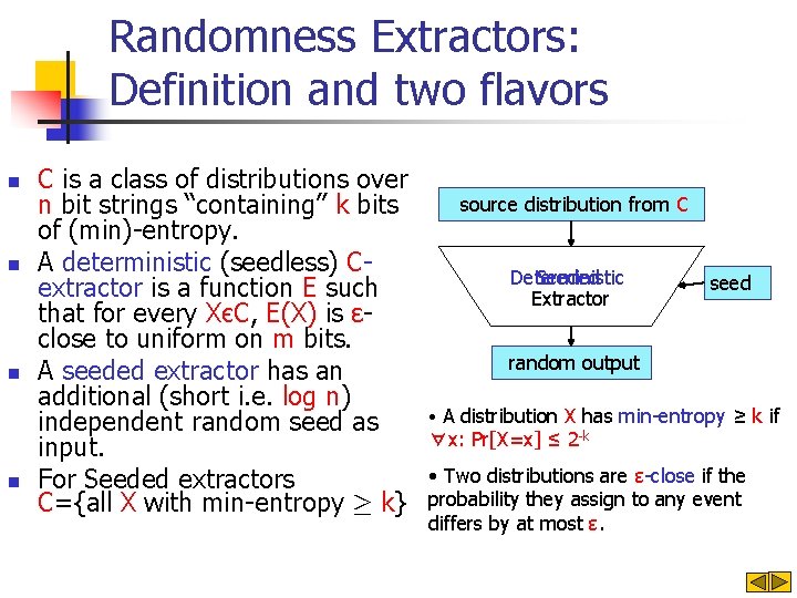
Randomness Extractors: Definition and two flavors n n C is a class of distributions over n bit strings “containing” k bits of (min)-entropy. A deterministic (seedless) Cextractor is a function E such that for every XєC, E(X) is εclose to uniform on m bits. A seeded extractor has an additional (short i. e. log n) independent random seed as input. For Seeded extractors C={all X with min-entropy ¸ k} source distribution from C Deterministic Seeded Extractor seed random output • A distribution X has min-entropy ≥ k if ∀x: Pr[X=x] ≤ 2 -k • Two distributions are ε-close if the probability they assign to any event differs by at most ε.

Zimand: explicit version of Yao’s lemma for decision trees Zimand defines and constructs a stronger variant of seeded extractors E(x, y) called “exposure resilient extractors”. He considers: B(x)=maj seeds y A(x, E(x, y)) Thm: [Zimand 07] If A is a randomized decision tree with q queries that tosses q random coins then: n B succeeds on most inputs. (a (1 -ρ)-fraction). n B can be implemented by a deterministic decision tree with q. O(1) queries. We improve to O(q) Zimand states his result a bit differently.

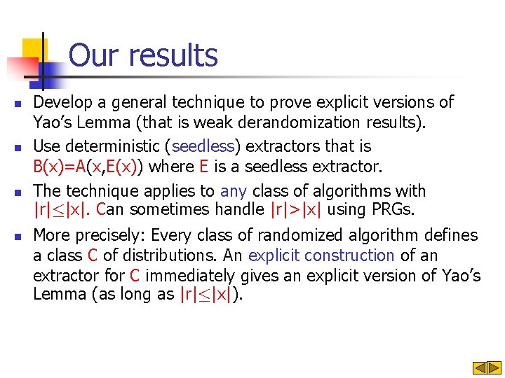
Our results n n Develop a general technique to prove explicit versions of Yao’s Lemma (that is weak derandomization results). Use deterministic (seedless) extractors that is B(x)=A(x, E(x)) where E is a seedless extractor. The technique applies to any class of algorithms with |r|·|x|. Can sometimes handle |r|>|x| using PRGs. More precisely: Every class of randomized algorithm defines a class C of distributions. An explicit construction of an extractor for C immediately gives an explicit version of Yao’s Lemma (as long as |r|·|x|).

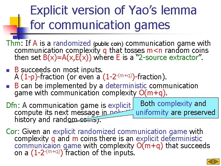
Explicit version of Yao’s lemma for communication games Thm: If A is a randomized (public coin) communication game with communication complexity q that tosses m<n random coins then set B(x)=A(x, E(x)) where E is a “ 2 -source extractor”. B succeeds on most inputs. A (1 -ρ)-fraction (or even a (1 -2 -(m+q))-fraction). n B can be implemented by a deterministic communication game with communication complexity O(m+q). Both party complexity Dfn: A communication game is explicit if each can and compute its next message in poly-time (given hisare input, uniformity preserved history and random coins). n Cor: Given an explicit randomized communication game with complexity q and m coins there is an explicit deterministic communicaion game with complexity O(m+q) that succeeds on a (1 -2 -(m+q)) fraction of the inputs.

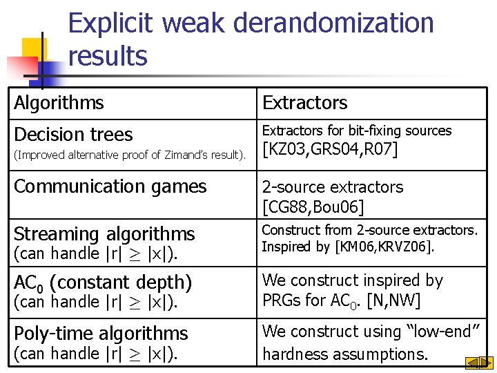
Explicit weak derandomization results Algorithms Extractors Decision trees Extractors for bit-fixing sources (Improved alternative proof of Zimand’s result). [KZ 03, GRS 04, R 07] Communication games 2 -source extractors [CG 88, Bou 06] Streaming algorithms Construct from 2 -source extractors. Inspired by [KM 06, KRVZ 06]. AC 0 (constant depth) We construct inspired by PRGs for AC 0. [N, NW] Poly-time algorithms We construct using “low-end” hardness assumptions. (can handle |r| ¸ |x|).

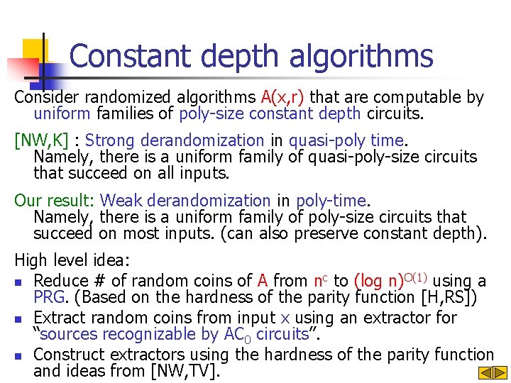
Constant depth algorithms Consider randomized algorithms A(x, r) that are computable by uniform families of poly-size constant depth circuits. [NW, K] : Strong derandomization in quasi-poly time. Namely, there is a uniform family of quasi-poly-size circuits that succeed on all inputs. Our result: Weak derandomization in poly-time. Namely, there is a uniform family of poly-size circuits that succeed on most inputs. (can also preserve constant depth). High level idea: n Reduce # of random coins of A from nc to (log n)O(1) using a PRG. (Based on the hardness of the parity function [H, RS]) n Extract random coins from input x using an extractor for “sources recognizable by AC 0 circuits”. n Construct extractors using the hardness of the parity function and ideas from [NW, TV].

High level overview of the proof To be concrete we consider communication games

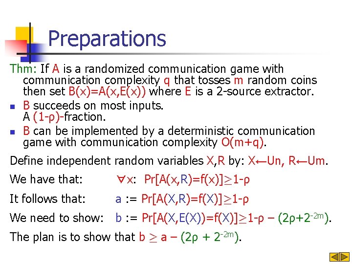
Preparations Thm: If A is a randomized communication game with communication complexity q that tosses m random coins then set B(x)=A(x, E(x)) where E is a 2 -source extractor. n B succeeds on most inputs. A (1 -ρ)-fraction. n B can be implemented by a deterministic communication game with communication complexity O(m+q). Define independent random variables X, R by: X←Un, R←Um. We have that: ∀x: Pr[A(x, R)=f(x)]¸ 1 -ρ It follows that: a : = Pr[A(X, R)=f(X)]¸ 1 -ρ We need to show: b : = Pr[A(X, E(X))=f(X)]¸ 1 -ρ – (2ρ+2 -2 m). The plan is to show that b ¸ a – (2ρ + 2 -2 m).

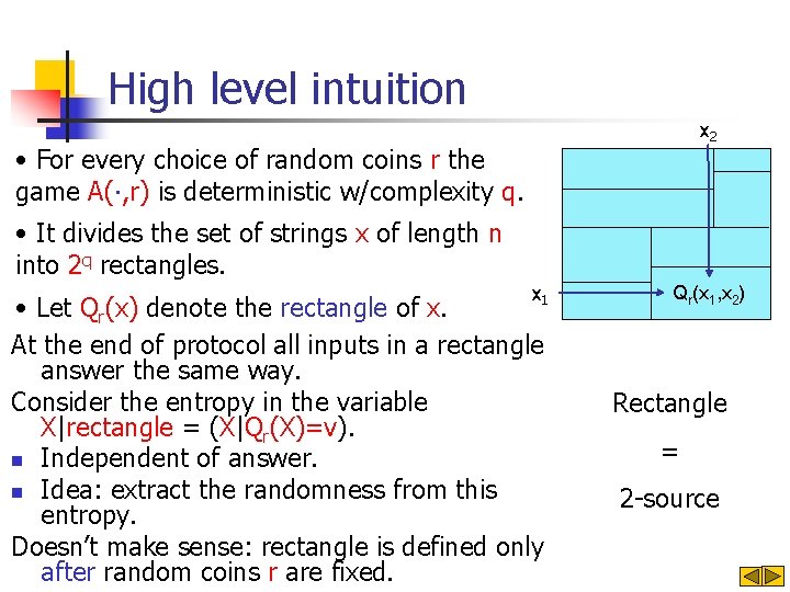
High level intuition x 2 • For every choice of random coins r the game A(∙, r) is deterministic w/complexity q. • It divides the set of strings x of length n into 2 q rectangles. x 1 • Let Qr(x) denote the rectangle of x. At the end of protocol all inputs in a rectangle answer the same way. Consider the entropy in the variable X|rectangle = (X|Qr(X)=v). n Independent of answer. n Idea: extract the randomness from this entropy. Doesn’t make sense: rectangle is defined only after random coins r are fixed. Qr(x 1, x 2) Rectangle = 2 -source

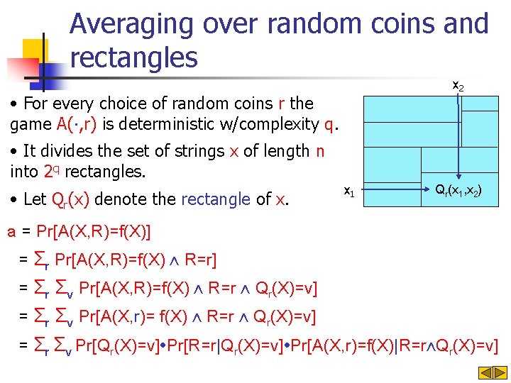
Averaging over random coins and rectangles x 2 • For every choice of random coins r the game A(∙, r) is deterministic w/complexity q. • It divides the set of strings x of length n into 2 q rectangles. • Let Qr(x) denote the rectangle of x. x 1 Qr(x 1, x 2) a = Pr[A(X, R)=f(X)] = Σr Pr[A(X, R)=f(X) ⋀ R=r] = Σr Σv Pr[A(X, R)=f(X) ⋀ R=r ⋀ Qr(X)=v] = Σr Σv Pr[A(X, r)= f(X) ⋀ R=r ⋀ Qr(X)=v] = Σr Σv Pr[Qr(X)=v]∙Pr[R=r|Qr(X)=v]∙Pr[A(X, r)=f(X)|R=r⋀Qr(X)=v]

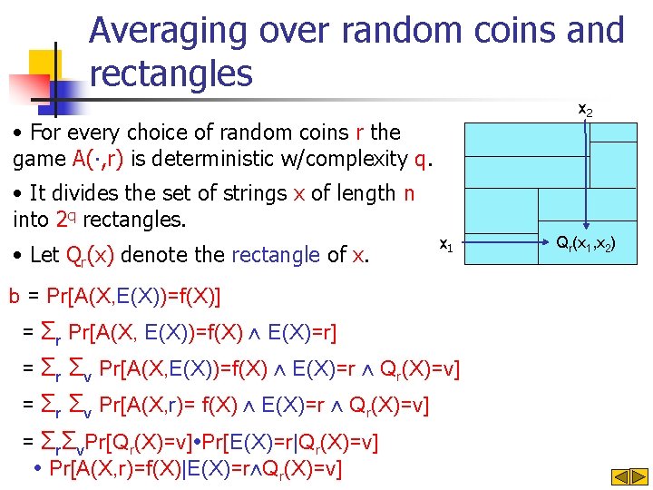
Averaging over random coins and rectangles x 2 • For every choice of random coins r the game A(∙, r) is deterministic w/complexity q. • It divides the set of strings x of length n into 2 q rectangles. • Let Qr(x) denote the rectangle of x. x 1 b = Pr[A(X, E(X))=f(X)] = Σr Pr[A(X, E(X))=f(X) ⋀ E(X)=r] = Σr Σv Pr[A(X, E(X))=f(X) ⋀ E(X)=r ⋀ Qr(X)=v] = Σr Σv Pr[A(X, r)= f(X) ⋀ E(X)=r ⋀ Qr(X)=v] = ΣrΣv. Pr[Qr(X)=v]∙Pr[E(X)=r|Qr(X)=v] ∙ Pr[A(X, r)=f(X)|E(X)=r⋀Qr(X)=v] Qr(x 1, x 2)

Proof (continued) a = Pr[A(X, R)=f(X)] ΣrΣv. Pr[Qr(X)=v]∙Pr[R=r |Qr(X)=v]∙Pr[A(X, r)=f(X)|R=r ⋀Qr(X)=v] ΣrΣv. Pr[Qr(X)=v]∙Pr[E(X)=r|Qr(X)=v]∙Pr[A(X, r)=f(X)|E(X)=r⋀Qr(X)=v] b = Pr[A(X, E(X))=f(X)]

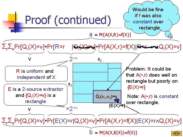
Would be fine if f was also constant over rectangle Proof (continued) a = Pr[A(X, R)=f(X)] ΣrΣv. Pr[Qr(X)=v]∙Pr[R=r |Qr(X)=v]∙Pr[A(X, r)=f(X)|R=r v 2 -m x 2 Problem: It could be that A( • , r) does well on rectangle but poorly on {E(X)=r} R is uniform and independent of X E is a 2 -source extractor and {Qr(X)=v} is a rectangle v ⋀Qr(X)=v] x 1 Qr(x 1, x 2)=v {E(X)=r} ≈2 -m Note: A( • , r) is constant over rectangle. ΣrΣv. Pr[Qr(X)=v]∙Pr[E(X)=r|Qr(X)=v]∙Pr[A(X, r)=f(X)|E(X)=r⋀Qr(X)=v] b = Pr[A(X, E(X))=f(X)]

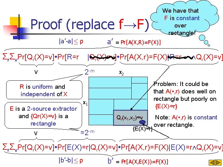
Modifying the argument We have that: Pr[A(X, R)=f(x)]¸ 1 -ρ By Yao’s lemma deterministic game F w/complexity q Pr[F(X)=f(X)]¸ 1 -ρ Consider randomized algorithm A’(x, r) which n Simulates A(x, r) n Simulates F(x) Let Qr(x) denote the rectangle of A’ and note that: • A(∙, r) is constant on rectangle {Qr(X)=v}. • F(x) is constant on rectangle {Qr(X)=v}.

Would be fine if f was also constant over rectangle Proof (continued) a = Pr[A(X, R)=f(X)] ΣrΣv. Pr[Qr(X)=v]∙Pr[R=r |Qr(X)=v]∙Pr[A(X, r)=f(X)|R=r v 2 -m x 2 Problem: It could be that A( • , r) does well on rectangle but poorly on {E(X)=r} R is uniform and independent of X E is a 2 -source extractor and {Qr(X)=v} is a rectangle v ⋀Qr(X)=v] x 1 Qr(x 1, x 2)=v {E(X)=r} ≈2 -m Note: A( • , r) is constant over rectangle. ΣrΣv. Pr[Qr(X)=v]∙Pr[E(X)=r|Qr(X)=v]∙Pr[A(X, r)=f(X)|E(X)=r⋀Qr(X)=v] b = Pr[A(X, E(X))=f(X)]

We have that F is constant over rectangle! Proof (replace f→F) a’ |a’-a|· ρ = Pr[A(X, R)=F(X)] ΣrΣv. Pr[Qr(X)=v]∙Pr[R=r |Qr(X)=v]∙Pr[A(X, r)=F(X)|R=r v 2 -m x 2 Problem: It could be that A( • , r) does well on rectangle but poorly on {E(X)=r} R is uniform and independent of X E is a 2 -source extractor and {Qr(X)=v} is a rectangle v ⋀Qr(X)=v] x 1 Qr(x 1, x 2)=v {E(X)=r} ≈2 -m Note: A( • , r) is constant over rectangle. ΣrΣv. Pr[Qr(X)=v]∙Pr[E(X)=r|Qr(X)=v]∙Pr[A(X, r)=F(X)|E(X)=r⋀Qr(X)=v] |b’-b|· ρ b’ = Pr[A(X, E(X))=F(X)]

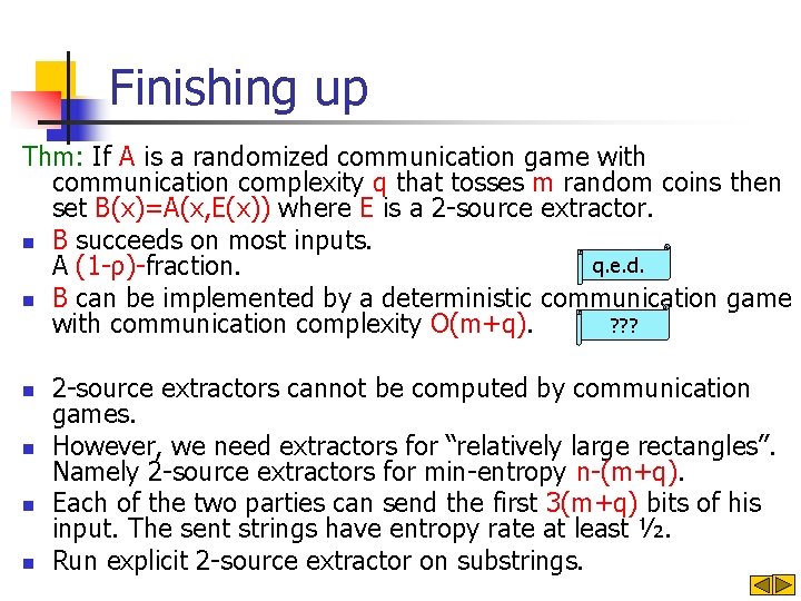
Finishing up Thm: If A is a randomized communication game with communication complexity q that tosses m random coins then set B(x)=A(x, E(x)) where E is a 2 -source extractor. n B succeeds on most inputs. q. e. d. A (1 -ρ)-fraction. n B can be implemented by a deterministic communication game ? ? ? with communication complexity O(m+q). n n 2 -source extractors cannot be computed by communication games. However, we need extractors for “relatively large rectangles”. Namely 2 -source extractors for min-entropy n-(m+q). Each of the two parties can send the first 3(m+q) bits of his input. The sent strings have entropy rate at least ½. Run explicit 2 -source extractor on substrings.

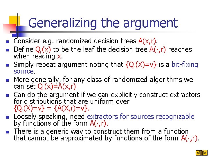
Generalizing the argument n n n n Consider e. g. randomized decision trees A(x, r). Define Qr(x) to be the leaf the decision tree A(∙, r) reaches when reading x. Simply repeat argument noting that {Qr(X)=v} is a bit-fixing source. More generally, for any class of randomized algorithms we can set Qr(x)=A(x, r) Can do the argument if we can explicitly construct extractors for distributions that are uniform over {Qr(X)=v} = {A(X, r)=v}. Loosely speaking, need extractors for sources recognizable by functions of the form A(∙, r). There is a generic way to construct them from a function that cannot be approximated by functions of the form A(∙, r).

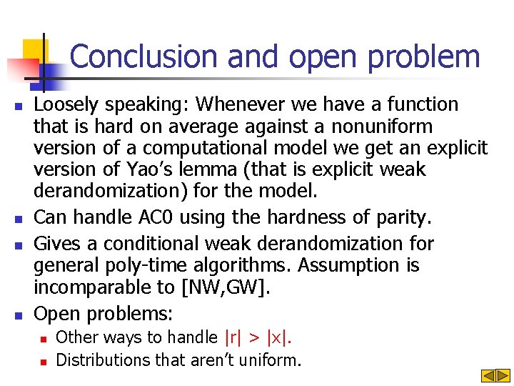
Conclusion and open problem n n Loosely speaking: Whenever we have a function that is hard on average against a nonuniform version of a computational model we get an explicit version of Yao’s lemma (that is explicit weak derandomization) for the model. Can handle AC 0 using the hardness of parity. Gives a conditional weak derandomization for general poly-time algorithms. Assumption is incomparable to [NW, GW]. Open problems: n n Other ways to handle |r| > |x|. Distributions that aren’t uniform.

That’s it…