Uncertainty in Sonar Performance Prediction A Probabilistic Approach

Uncertainty in Sonar Performance Prediction: A Probabilistic Approach Applied to East China Sea Operations Phil Abbot, OASIS Inc. ONR QPE Uncertainty DRI 1 st Mtg San Francisco, CA 8 December 2006

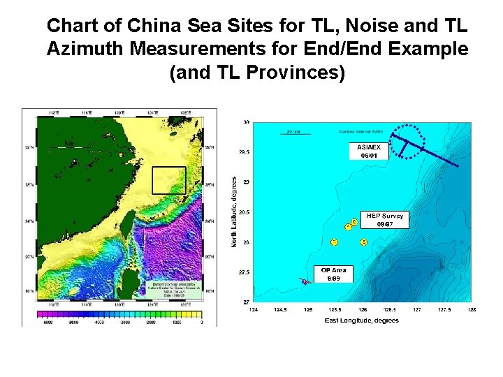
Chart of China Sea Sites for TL, Noise and TL Azimuth Measurements for End/End Example (and TL Provinces)

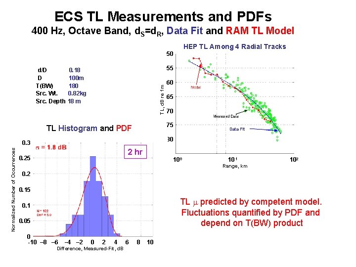
ECS TL Measurements and PDFs 400 Hz, Octave Band, d. S=d. R, Data Fit and RAM TL Model HEP TL Among 4 Radial Tracks 50 55 TL, d. B re 1 m d/D 0. 18 D 100 m T(BW) 180 Src. Wt. 0. 82 kg Src. Depth 18 m 65 70 75 TL Histogram and PDF Data Fit 80 0. 3 Normalized Number of Occurrences 60 2 hr 0. 25 100 10 1 Range, km 102 0. 15 TL predicted by competent model. Fluctuations quantified by PDF and depend on T(BW) product 0. 1 0. 05 0 -10 – 8 – 6 – 4 – 2 0 2 4 Difference, Measured-Fit, d. B 6 8 10

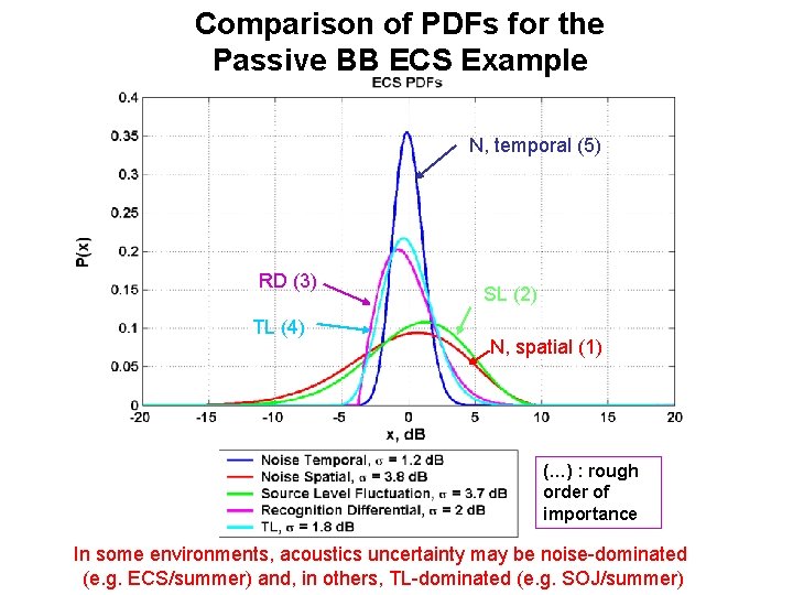
Comparison of PDFs for the Passive BB ECS Example N, temporal (5) RD (3) TL (4) SL (2) N, spatial (1) (…) : rough order of importance In some environments, acoustics uncertainty may be noise-dominated (e. g. ECS/summer) and, in others, TL-dominated (e. g. SOJ/summer)

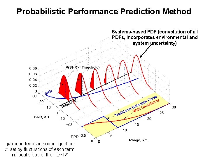
Probabilistic Performance Prediction Method Systems-based PDF (convolution of all PDFs, incorporates environmental and system uncertainty) : mean terms in sonar equation : set by fluctuations of each term n: local slope of the TL~ Rn

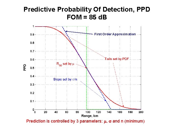
Predictive Probability Of Detection, PPD FOM = 85 d. B First Order Approximation Prediction is controlled by 3 parameters: , and n (minimum)

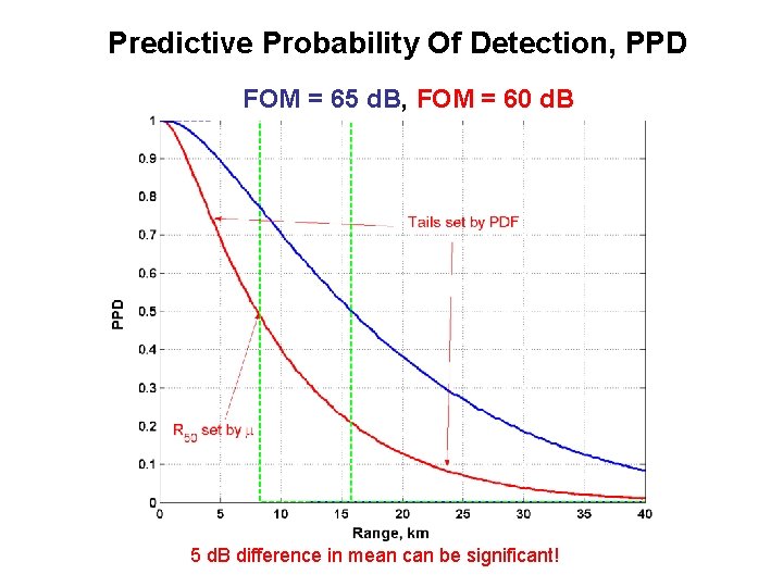
Predictive Probability Of Detection, PPD FOM = 65 d. B, FOM = 60 d. B 5 d. B difference in mean can be significant!

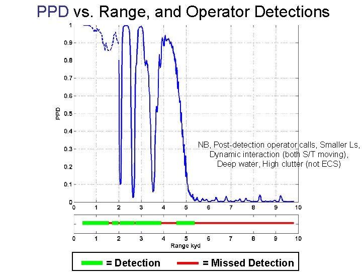
PPD vs. Range, and Operator Detections NB, Post-detection operator calls, Smaller Ls, Dynamic interaction (both S/T moving), Deep water, High clutter (not ECS) = Detection = Missed Detection

Summary • Probabilistic performance prediction reasonably represents the sonar/target system for both BB and NB examples • TL set primarily by macro state of ocean (w/bottom) – Determined by numerous samples of measured TL (or improved estimates of ocean) or from fewer TL samples assimilated with a competent TL model • TL and PDF set by micro state of ocean (temporal/spatial “graininess”) • Measurements in probabilistic framework that supplement propagation and environmental (ocean and bottom) models (i. e. data assimilation) for SW, rather than models alone, are necessary for competent prediction

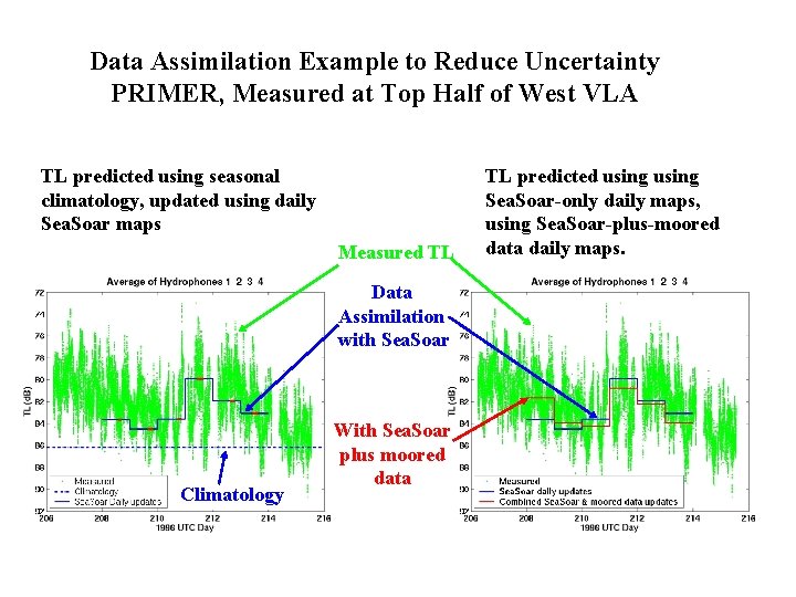
Data Assimilation Example to Reduce Uncertainty PRIMER, Measured at Top Half of West VLA TL predicted using seasonal climatology, updated using daily Sea. Soar maps Measured TL Data Assimilation with Sea. Soar Climatology With Sea. Soar plus moored data TL predicted using Sea. Soar-only daily maps, using Sea. Soar-plus-moored data daily maps.

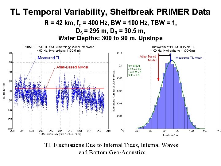
TL Temporal Variability, Shelfbreak PRIMER Data R = 42 km, fc = 400 Hz, BW = 100 Hz, TBW = 1, DS = 295 m, DR = 30. 5 m, Water Depths: 300 to 90 m, Upslope PRIMER Peak TL and Climatology Model Prediction 400 Hz, Hydrophone 1 (30. 5 m) Histogram of PRIMER Peak TL 400 Hz, Hydrophone 1 (30. 5 m) Atlas-Based Model Measured TL Mean TL Fluctuations Due to Internal Tides, Internal Waves and Bottom Geo-Acoustics

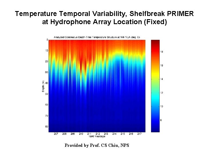
Temperature Temporal Variability, Shelfbreak PRIMER at Hydrophone Array Location (Fixed) Provided by Prof. CS Chiu, NPS

Backups

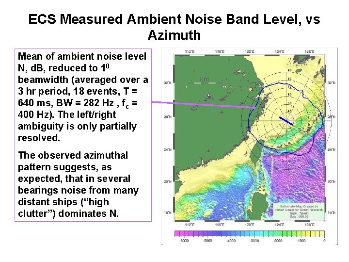
ECS Measured Ambient Noise Band Level, vs Azimuth Mean of ambient noise level N, d. B, reduced to 10 beamwidth (averaged over a 3 hr period, 18 events, T = 640 ms, BW = 282 Hz , fc = 400 Hz). The left/right ambiguity is only partially resolved. The observed azimuthal pattern suggests, as expected, that in several bearings noise from many distant ships (“high clutter”) dominates N.

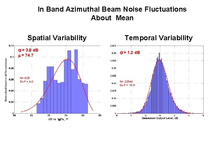
In Band Azimuthal Beam Noise Fluctuations About Mean Spatial Variability = 3. 8 d. B Temporal Variability = 1. 2 d. B = 74. 7 N= 629 Do. F = 4. 0 N= 22544 Do. F = 16. 9 d. B re 1 Pa, 1 o

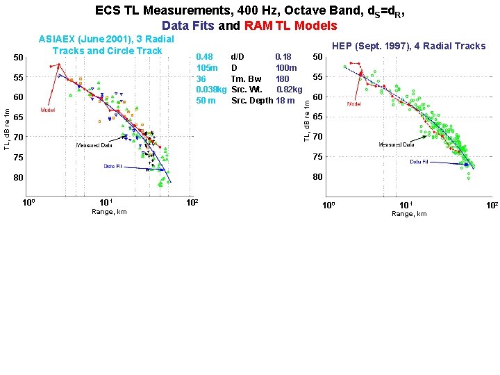
ECS TL Measurements, 400 Hz, Octave Band, d. S=d. R, Data Fits and RAM TL Models 55 TL, d. B re 1 m 60 HEP (Sept. 1997), 4 Radial Tracks 0. 48 105 m 36 0. 038 kg 50 m 65 70 d/D 0. 18 D 100 m Tm. Bw 180 Src. Wt. 0. 82 kg Src. Depth 18 m TL, d. B re 1 m 50 ASIAEX (June 2001), 3 Radial Tracks and Circle Track 50 55 60 65 70 75 75 80 80 10 1 Range, km 102 100 10 1 Range, km 102

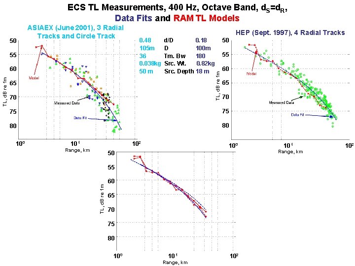
ECS TL Measurements, 400 Hz, Octave Band, d. S=d. R, Data Fits and RAM TL Models 55 0. 48 105 m 36 0. 038 kg 50 m d/D 0. 18 D 100 m Tm. Bw 180 Src. Wt. 0. 82 kg Src. Depth 18 m 65 70 50 55 60 65 70 75 75 80 80 10 1 102 Range, km 100 50 55 TL, d. B re 1 m 60 HEP (Sept. 1997), 4 Radial Tracks TL, d. B re 1 m 50 ASIAEX (June 2001), 3 Radial Tracks and Circle Track 60 65 70 75 80 10 1 Range, km 102

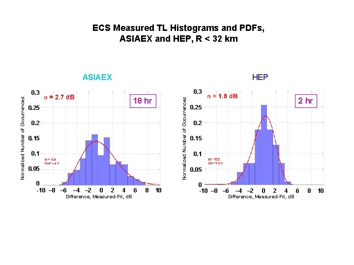
ECS Measured TL Histograms and PDFs, ASIAEX and HEP, R < 32 km HEP ASIAEX 0. 3 18 hr 0. 25 Normalized Number of Occurrences 0. 3 0. 2 0. 15 0. 1 0. 05 0 -10 – 8 – 6 – 4 – 2 0 2 4 Difference, Measured-Fit, d. B 6 8 10 2 hr 0. 25 0. 2 0. 15 0. 1 0. 05 0 -10 – 8 – 6 – 4 – 2 0 2 4 Difference, Measured-Fit, d. B 6 8 10

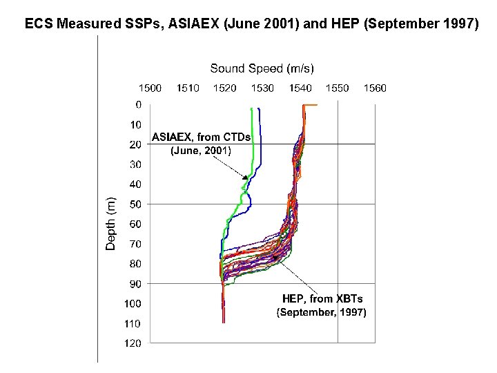
ECS Measured SSPs, ASIAEX (June 2001) and HEP (September 1997)

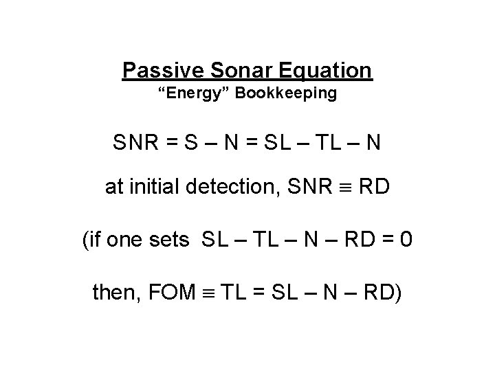
Passive Sonar Equation “Energy” Bookkeeping SNR = S – N = SL – TL – N at initial detection, SNR RD (if one sets SL – TL – N – RD = 0 then, FOM TL = SL – N – RD)

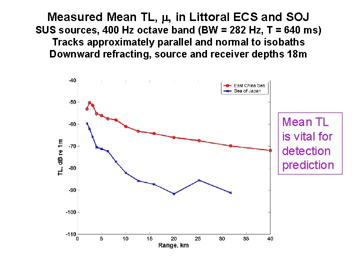
Measured Mean TL, , in Littoral ECS and SOJ SUS sources, 400 Hz octave band (BW = 282 Hz, T = 640 ms) Tracks approximately parallel and normal to isobaths Downward refracting, source and receiver depths 18 m Mean TL is vital for detection prediction

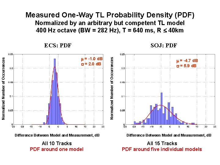
Measured One-Way TL Probability Density (PDF) Normalized by an arbitrary but competent TL model 400 Hz octave (BW = 282 Hz), T = 640 ms, R 40 km SOJ: PDF = -1. 0 d. B = 2. 0 d. B Difference Between Model and Measurement, d. B All 10 Tracks PDF around one model Normalized Number of Occurrences ECS: PDF = -4. 7 d. B = 5. 9 d. B Difference Between Model and Measurement, d. B All 15 Tracks PDF around five individual models

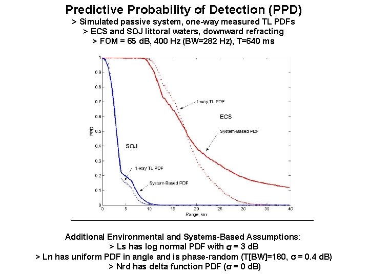
Predictive Probability of Detection (PPD) > Simulated passive system, one-way measured TL PDFs > ECS and SOJ littoral waters, downward refracting > FOM = 65 d. B, 400 Hz (BW=282 Hz), T=640 ms Additional Environmental and Systems-Based Assumptions: > Ls has log normal PDF with = 3 d. B > Ln has uniform PDF in angle and is phase-random (T[BW]=180, = 0. 4 d. B) > Nrd has delta function PDF ( = 0 d. B)

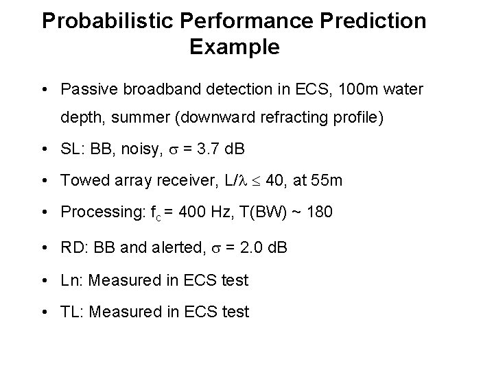
Probabilistic Performance Prediction Example • Passive broadband detection in ECS, 100 m water depth, summer (downward refracting profile) • SL: BB, noisy, = 3. 7 d. B • Towed array receiver, L/ 40, at 55 m • Processing: fc = 400 Hz, T(BW) ~ 180 • RD: BB and alerted, = 2. 0 d. B • Ln: Measured in ECS test • TL: Measured in ECS test