UMass Lowell Computer Science 91 504 Advanced Algorithms

UMass Lowell Computer Science 91. 504 Advanced Algorithms Computational Geometry Prof. Karen Daniels Spring, 2010 O’Rourke Chapter 6 with some material from de Berg et al. Chapter 8 Arrangements

Chapter 6 Arrangements Introduction Combinatorics of Arrangements Incremental Algorithm Three and Higher Dimensions Duality Higher-Order Voronoi Diagrams Applications

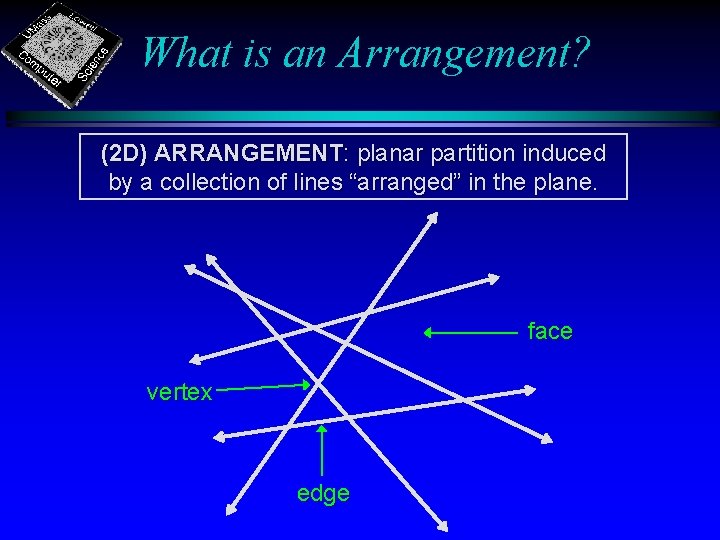
What is an Arrangement? (2 D) ARRANGEMENT: planar partition induced by a collection of lines “arranged” in the plane. face vertex edge

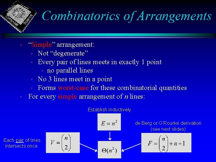
Combinatorics of Arrangements • • “Simple” arrangement: • Not “degenerate” • Every pair of lines meets in exactly 1 point • no parallel lines • No 3 lines meet in a point • Forms worst-case for these combinatorial quantities For every simple arrangement of n lines: Establish inductively. de Berg or O’Rourke derivation (see next slides) Each pair of lines intersects once.

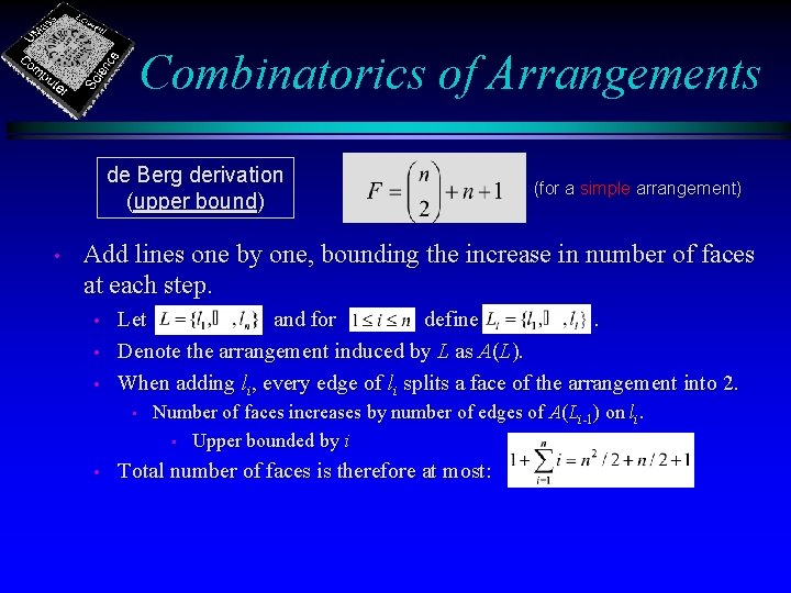
Combinatorics of Arrangements de Berg derivation (upper bound) • (for a simple arrangement) Add lines one by one, bounding the increase in number of faces at each step. • • • Let and for define. Denote the arrangement induced by L as A(L). When adding li, every edge of li splits a face of the arrangement into 2. • • Number of faces increases by number of edges of A(Li-1 i-1) on li. • Upper bounded by i Total number of faces is therefore at most:

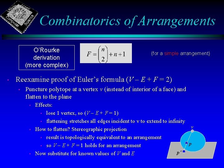
Combinatorics of Arrangements O’Rourke derivation (more complex) • (for a simple arrangement) Reexamine proof of Euler’s formula (V – E + F = 2) • Puncture polytope at a vertex v (instead of interior of a face) and flatten to the plane • • • Effects: • lose 1 vertex, so (V – E + F = 1) • flattening stretches all edges incident to v to extend to infinity v How to flatten? Stereographic projection • result is topologically equivalent to an arrangement p • so V – E + F = 1 holds for an arrangement p’ Now substitute for known values of V and E

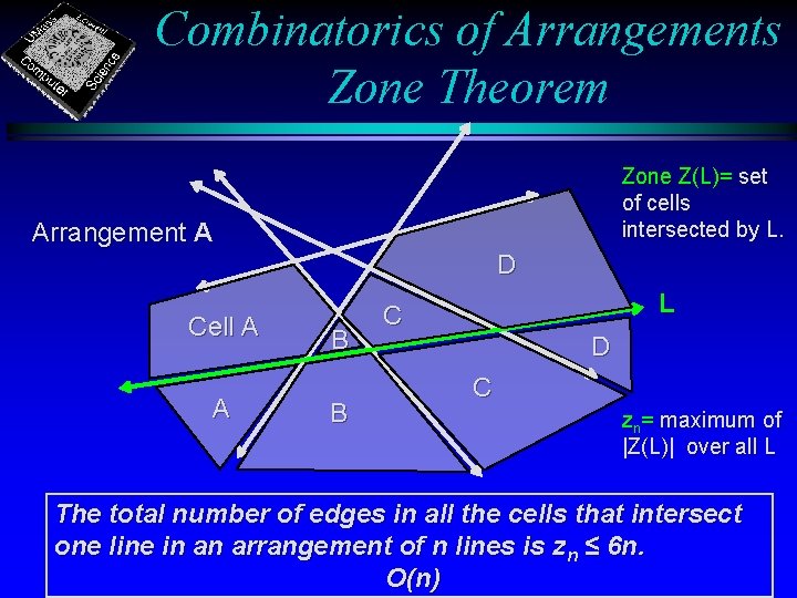
Combinatorics of Arrangements Zone Theorem Zone Z(L)= set of cells intersected by L. Arrangement A D Cell A A B B L C D C zn= maximum of |Z(L)| over all L The total number of edges in all the cells that intersect one line in an arrangement of n lines is zn ≤ 6 n. O(n)

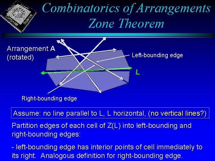
Combinatorics of Arrangements Zone Theorem Arrangement A (rotated) Left-bounding edge L Right-bounding edge Assume: no line parallel to L, L horizontal, (no vertical lines? ) Partition edges of each cell of Z(L) into left-bounding and right-bounding edges: - left-bounding edge has interior points of cell immediately to its right. Analogous definition for right-bounding edge.

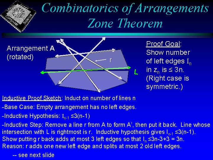
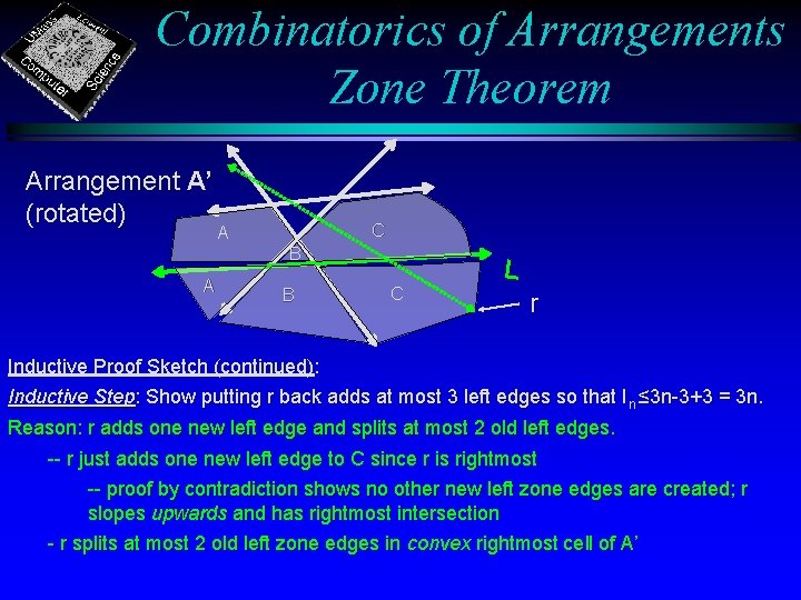
Combinatorics of Arrangements Zone Theorem Arrangement A (rotated) r L Proof Goal: Show number of left edges In in zn is ≤ 3 n. (Right case is symmetric. ) Inductive Proof Sketch: Induct on number of lines n -Base Case: Empty arrangement has no left edges. -Inductive Hypothesis: In-1 ≤ 3(n-1) -Inductive Step: Remove a line r from A to form A’, then put it back. Line whose intersection with L is rightmost is r. Inductive hypothesis gives In-1 ≤ 3(n-1). Show putting r back adds at most 3 left edges so that In ≤ 3 n-3+3 = 3 n. Reason: r adds one new left edge and splits at most 2 old left edges. -- see next slide

Combinatorics of Arrangements Zone Theorem Arrangement A’ (rotated) C A B C L r Inductive Proof Sketch (continued): Inductive Step: Show putting r back adds at most 3 left edges so that In ≤ 3 n-3+3 = 3 n. Reason: r adds one new left edge and splits at most 2 old left edges. -- r just adds one new left edge to C since r is rightmost -- proof by contradiction shows no other new left zone edges are created; r slopes upwards and has rightmost intersection - r splits at most 2 old left zone edges in convex rightmost cell of A’

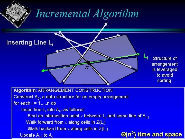
Incremental Algorithm Inserting Line Li Li x Algorithm: ARRANGEMENT CONSTRUCTION Construct A 0, a data structure for an empty arrangement for each i = 1, . . . , n do Insert line Li into Ai-1 as follows: Find an intersection point x between Li and some line of Ai-1 Walk forward from x along cells in Z(Li) Walk backard from x along cells in Z(Li) Q(n 2) time Update Ai-1 to Ai Structure of arrangement is leveraged to avoid sorting. and space

Three and Higher Dimensions • • 2 D results extend to higher dimensions For an arrangement of hyperplanes in d dimensions • • • number of faces is O(nd) zone of a hyperplane has complexity O(nd-1) construct in O(nd) time and space

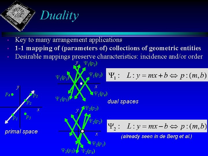
Duality • • • Key to many arrangement applications 1 -1 mapping of (parameters of) collections of geometric entities Desirable mappings preserve characteristics: incidence and/or order y Y 1(p 2) Y 1(p 1) x y p 4 p 3 p 2 Y 1(p 3) Y 1(p 4) y Y 2(p 5) x p 1 Y 1(p 5) p 5 dual spaces Y 2(p 2) primal space x Y 2(p 3) Y 2(p 1) Y 2(p 4) (already seen in de Berg et al. )

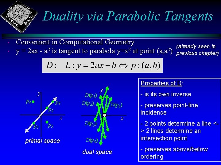
Duality via Parabolic Tangents • • Convenient in Computational Geometry y = 2 ax - a 2 is tangent to parabola y=x 2 at point (a, a 2) y p 4 p 3 p 2 x p 1 p 5 primal space D(p 1) D(p 4) (already seen in previous chapter) Properties of D: y - is its own inverse D(p 2) D(p 5) D(p 3) dual space x - preserves point-line incidence - 2 points determine a line <> 2 lines determine an intersection point - preserves above/below ordering

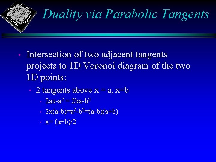
Duality via Parabolic Tangents • Intersection of two adjacent tangents projects to 1 D Voronoi diagram of the two 1 D points: • 2 tangents above x = a, x=b • • • 2 ax-a 2 = 2 bx-b 2 2 x(a-b)=a 2 -b 2=(a-b)(a+b) x= (a+b)/2

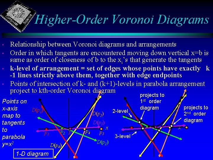
Higher-Order Voronoi Diagrams • • Relationship between Voronoi diagrams and arrangements Order in which tangents are encountered moving down vertical x=b is same as order of closeness of b to the xi’s that generate the tangents k-level of arrangement = set of edges whose points have exactly k -1 lines strictly above them, together with edge endpoints Points of intersection of k- and (k+1)-levels in parabola arrangement project to kth-order Voronoi diagram Points on x-axis D(p 1) map to tangents to p 2 p 3 p 1 parabola y=x 2 D(p 4) 1 -D diagram 2 -level D(p 5) D(p 3) p 4 p 5 projects to 2 nd order diagram x x D(p 2) projects to 1 st order diagram 3 -level

Applications • K-Nearest Neighbors • • Hidden Surface Removal for Graphics • • characteristic views an object can present to viewer (combinatorially equivalent) Smallest Polytope Shadow • • topological sweep of arrangement of objects Aspect Graphs for Computer Vision • • kth order Voronoi diagram can be used to find k-nearest neighbors of query point combinatorial structure of shadow projection changes when viewpoint crosses a plane Ham-Sandwich Cuts of a Point Set • • bisector of point set is line having at most ½ points strictly to each side bisectors of point set dualize to median level of dual line arrangement all ham-sandwich cuts for sets A, B: intersect median levels of A, B higher dimensional generalization: for d point sets in d dimensions, there exists a hyperplane simultaneously bisecting each point set

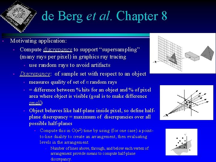
de Berg et al. Chapter 8 • Motivating application: • Compute discrepancy to support “supersampling” (many rays per pixel) in graphics ray tracing • use random rays to avoid artifacts • Discrepancy: of sample set with respect to an object • • • measures quality of set of n random rays = difference between % hits for an object and % of pixel area where object is visible (goal is to make difference small) Object behaves like half-plane inside pixel, so define halfplane discrepancy = maximum of discrepancies over all possible half-planes • Compute this in O(n 2) time by using (for one case) a pointto-line duality to create an arrangement, then evaluating levels in the arrangement. • Number of lines above, through, and below each vertex of arrangement provide means to compute half-plane discrepancy.