Uhlkov cyklus Sklenkov plyny Radian psoben Antropogenn emise

Uhlíkový cyklus Skleníkové plyny Radiační působení Antropogenní emise skleníkových plynů a perturbace uhlíkového cyklu Scénáře emisí Mezinárodní aktivity a závazky

Přirozené a antropogenní změny klimatu Po většinu času se změny klimatu odehrávaly bez přítomnosti člověka, proto je také někdy nazýváme přirozenými změnami na rozdíl od tzv. změn antropogenních, na kterých má podíl člověk. V období přístrojových měření se na přirozeném kolísání klimatu mohla podílet zejména sluneční činnost, přirozené aerosoly (např. aerosoly spojené s vulkanickou činností) a vzájemné působení atmosféry a oceánu. Člověk od počátku své existence ovlivňuje své okolí. Nejprve v blízkosti svých sídel, později na větších územích. Kácel stromy, vypaloval křoviny a travnaté porosty, obdělával stále více půdy, pásl dobytek - měnil charakter krajiny. Zasahoval tak do vodní bilance zemského povrchu, měnil jeho albedo i složení atmosféry.

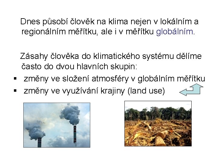
Dnes působí člověk na klima nejen v lokálním a regionálním měřítku, ale i v měřítku globálním. Zásahy člověka do klimatického systému dělíme často do dvou hlavních skupin: § změny ve složení atmosféry v globálním měřítku § změny ve využívání krajiny (land use)

Výhled do budoucna Klíčové otázky: a) jak porostou emise a koncentrace skleníkových plynů a aerosolů v budoucích letech, tedy mj. jakou cestou se bude ubírat vývoj lidské společnosti b) jaká bude reakce klimatického systému na růst koncentrací skleníkových plynů a aerosolů v atmosféře Ve výhledech není zahrnut vliv vnějších faktorů na klimatický systém

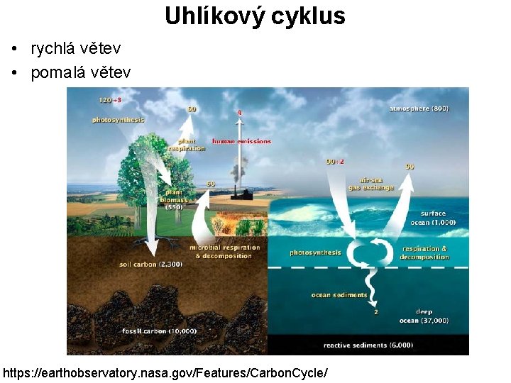
Uhlíkový cyklus • rychlá větev • pomalá větev https: //earthobservatory. nasa. gov/Features/Carbon. Cycle/

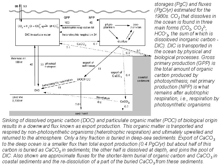
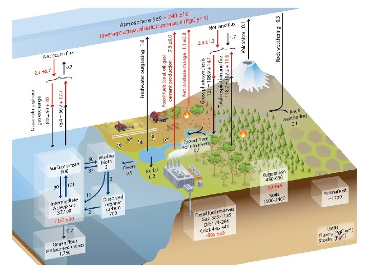
storages (Pg. C) and fluxes (Pg. C/yr) estimated for the 1980 s. CO 2 that dissolves in the ocean is found in three main forms (CO 2, CO 32 -, HCO-3, the sum of which is dissoloved inorganic carbon DIC). DIC is transported in the ocean by physical and biological processes. Gross primary production (GPP) is the total amount of organic carbon produced by photosynthesis; net primary production (NPP) is what remains after autotrophic respiration, i. e. , respiration by photosynthetic organisms. Sinking of dissolved organic carbon (DOC) and particulate organic matter (POC) of biological origin results in a downward flux known as export production. This organic matter is tranported and respired by non-photosynthetic organisms (heterotrophic respiration) and ultimately upwelled and returned to the atmosphere. Only a tiny fraction is buried in deep-sea sediments. Export of Ca. CO 3 to the deep ocean is a smaller flux than total export production (0. 4 Pg. C/yr) but about half of this carbon is buried as Ca. CO 3 in sediments; the other half is dissolved at depth, and joins the pool of DIC. Also shown are approximate fluxes for the shorter-term burial of organic carbon and Ca. CO 3 in coastal sediments and the re-dissolution of a part of the buried Ca. CO 3 from these sediments.

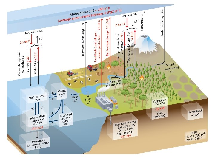
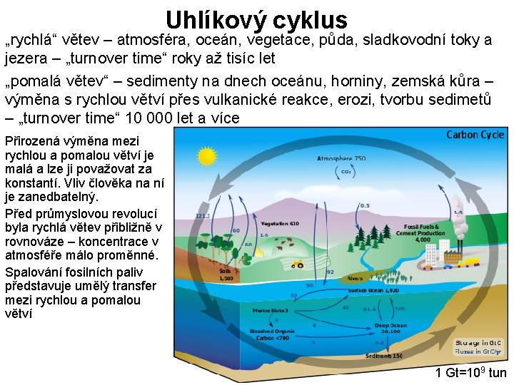
Uhlíkový cyklus „rychlá“ větev – atmosféra, oceán, vegetace, půda, sladkovodní toky a jezera – „turnover time“ roky až tisíc let „pomalá větev“ – sedimenty na dnech oceánu, horniny, zemská kůra – výměna s rychlou větví přes vulkanické reakce, erozi, tvorbu sedimetů – „turnover time“ 10 000 let a více Přirozená výměna mezi rychlou a pomalou větví je malá a lze ji považovat za konstantí. Vliv člověka na ní je zanedbatelný. Před průmyslovou revolucí byla rychlá větev přibližně v rovnováze – koncentrace v atmosféře málo proměnné. Spalování fosilních paliv představuje umělý transfer mezi rychlou a pomalou větví 1 Gt=109 tun

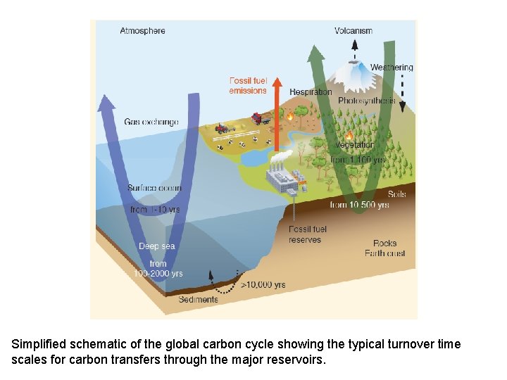
Simplified schematic of the global carbon cycle showing the typical turnover time scales for carbon transfers through the major reservoirs.

Skleníkové plyny (GHG) Při spalování fosilních paliv, kácení lesů, vypalování savan, při zemědělské výrobě, dopravě a v důsledku mnoha dalších průmyslových aktivit se do atmosféry uvolňují plyny, které buď přímo, nebo prostřednictvím látek, vznikajících při jejich chemických reakcích, zesilují přirozený skleníkový efekt atmosféry. Hlavní antropogenní skleníkové plyny: oxid uhličitý (CO 2), troposférický ozón (O 3), metan (CH 4), oxid dusný (N 2 O), fluorované uhlovodíky (HFC), perfluorované uhlovodíky (PFC), fluorid sírový (SF 6) Látky narušující ozonovou vrstvu: plně chlorované a fluorované uhlovodíky (CFC), neúplně chlorované a fluorované uhlovodíky (HCFC) a halony. • Změny koncentrací skleníkových plynů a aerosolů mění energetickou bilanci klimatického systému - zásah do dalších procesů prostřednictvím zpětných vazeb.

Názvosloví Chlor-fluorované uhlovodíky (CFC - chlorofluorocarbon) halogenderiváty uhlovodíků, v nichž alespoň jeden radikál je fluor (fluorované uhlovodíky) nebo chlor (chlorované uhlovodíky). Jejich nejznámější podskupinou jsou freony Perfluorované uhlovodíky (PFC) sloučeniny, které ve své molekule obsahují pouze atomy uhlíku a fluoru, např. perfluorometan Fluorid sírový (SF 6) úplně chlorované a fluorované uhlovodíky (CFCs) částečně chlorované a fluorované uhlovodíky (HCFCs) halony (obsahují brom) • ppm - parts per million, tzn. počet objemových částí sledované plynné látky v milionu objemových částí vzduchu. • ppb - parts per billion, 1 ppb = 10 -3 ppm • ppt - parts per trillion 1 ppt = 10 -12

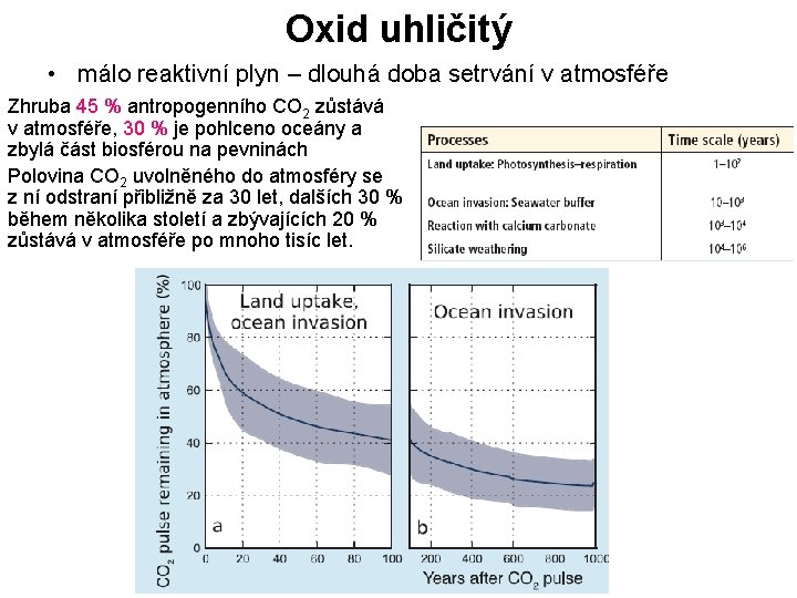
Oxid uhličitý • málo reaktivní plyn – dlouhá doba setrvání v atmosféře Zhruba 45 % antropogenního CO 2 zůstává v atmosféře, 30 % je pohlceno oceány a zbylá část biosférou na pevninách Polovina CO 2 uvolněného do atmosféry se z ní odstraní přibližně za 30 let, dalších 30 % během několika století a zbývajících 20 % zůstává v atmosféře po mnoho tisíc let.

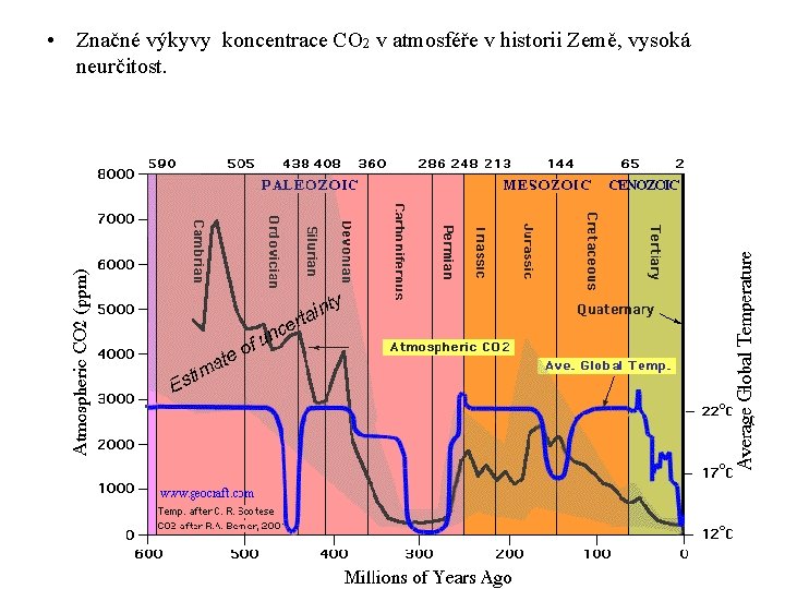
• Značné výkyvy koncentrace CO 2 v atmosféře v historii Země, vysoká neurčitost.

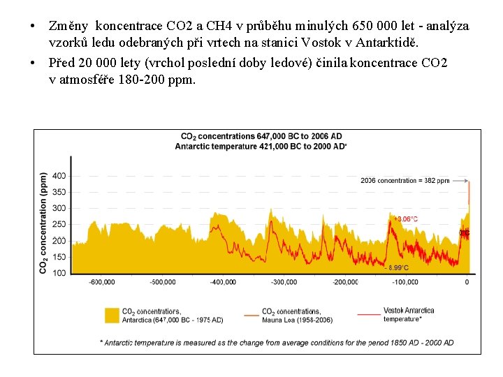
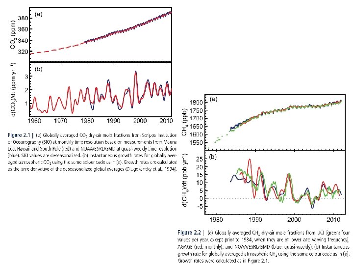
• Změny koncentrace CO 2 a CH 4 v průběhu minulých 650 000 let - analýza vzorků ledu odebraných při vrtech na stanici Vostok v Antarktidě. • Před 20 000 lety (vrchol poslední doby ledové) činila koncentrace CO 2 v atmosféře 180 -200 ppm.

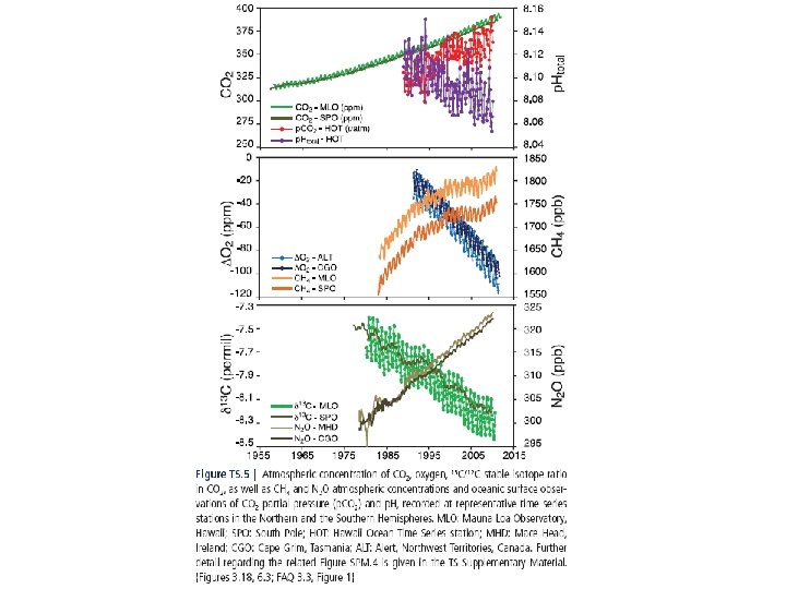
• Poslední tisíciletí: – koncentrace CO 2 prakticky konstantní – 1000– 1750 n. l. : rozmezí 275– 285 ppm • od poloviny 18. století začíná postupný růst koncentrace • Posledních 250 let: – zvýšení koncentrace CO 2 o 100 ppm (36 %) – 379 ppm v roce 2005 – 400 ppm v lednu 2015 • Současná hodnota pravděpodobně nejvyšší, jaké bylo za uplynulých 650 tisíc let dosaženo. • Meziroční proměnlivost: – zřejmě zejména vliv variability klimatu, např. El-Niño, v jejímž důsledku dochází ke změnám uvolňování a pohlcování CO 2 oceány a na pevninách. • Růst CO 2 způsoben oxidací organického uhlíku (hořením fosilních paliv) – důkazy ve složení izotopů CO 2 a pozorovaný úbytek O 2

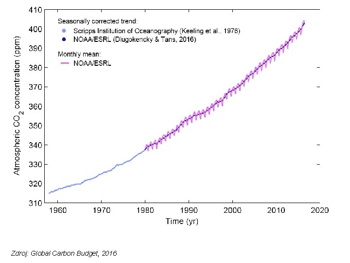
Zdroj: Global Carbon Budget, 2016

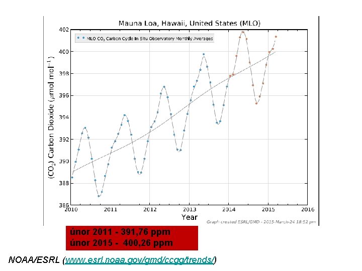
únor 2011 - 391, 76 ppm únor 2015 - 400, 26 ppm NOAA/ESRL (www. esrl. noaa. gov/gmd/ccgg/trends/)

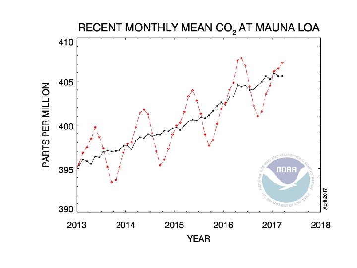
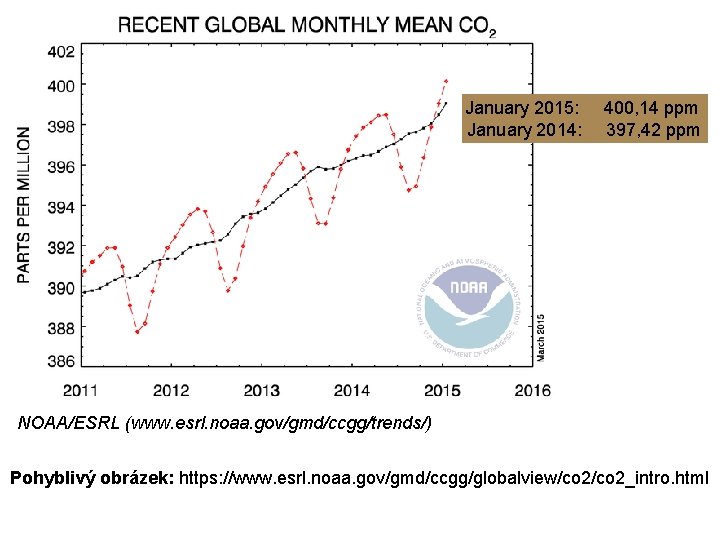
January 2015: 400, 14 ppm January 2014: 397, 42 ppm NOAA/ESRL (www. esrl. noaa. gov/gmd/ccgg/trends/) Pohyblivý obrázek: https: //www. esrl. noaa. gov/gmd/ccgg/globalview/co 2_intro. html

NOAA/ESRL calculation of global means • http: //www. esrl. noaa. gov/gmd/ccgg/about/global_means. html

Metan • zdroje přírodní (např. mokřiny, termiti, oceány) i antropogenní (těžba a transport uhlí, zemního plynu, chov zvířectva, skládky a odpadní vody, hospodaření se živočišným odpadem, pěstování rýže) • • Více než polovina dnešních emisí je antropogenního původu. Z atmosféry je metan odstraňován chemickými reakcemi. Relativně krátká doba setrvání v atmosféře (v průměru 12 let) Globální atmosférická koncentrace: – předindustriální hodnota zhruba 715 ppb – začátkem 90. let 1732 ppb a v roce 2005 1774 ppb. • Koncentrace v roce 2005 výrazně přesáhla rozsah hodnot za posledních 650 000 let (320 až 790 ppb), zrekonstruovaný z ledových vrtů. • Rychlost nárůstu od počátku 90. let poklesla, což je v souladu s tím, že celkový objem emisí (z antropogenních i přirozených zdrojů) byl v průběhu tohoto období takřka konstantní. • Je velmi pravděpodobné, že pozorovaný nárůst koncentrací metanu je důsledkem lidské činnosti, převážně zemědělské výroby a využívání fosilních paliv, relativní příspěvky různých typů zdrojů nejsou ale dobře určeny. Navíc není zcela jasný vývoj od počátku 90. let, konkrétně není zcela jasné proč se koncentrace od té doby příliš nemění.

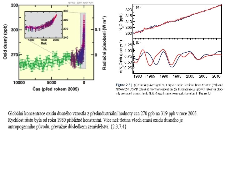
Oxid dusný • emise při zemědělských a průmyslových aktivitách (používání dusíkatých hnojiv), při spalování fosilních paliv (kouřové vlečky elektráren) a pevného odpadu. • Doba setrvání v atmosféře asi 120 let. • Globální koncentrace: – předindustriální hodnoty cca 270 ppb – 319 ppb v roce 2005 – 324 ppb v roce 2011. • Rychlost růstu od roku 1980 přibližně konstantní. • Zhruba 40 % všech emisí oxidu dusného je antropogenního původu, převážně důsledkem zemědělské výroby. • Nesnadnost kvantifikace antropogenních i přirozených zdrojů. • Z atmosféry je N 2 O uvolňován chemickými reakcemi, ve stratosféře fotochemickými. • Sezónní změny koncentrací jsou dány zejména úniky do stratosféry. • N 2 O je momentálně třetím GHG co do příspěvku k radiačnímu působení.

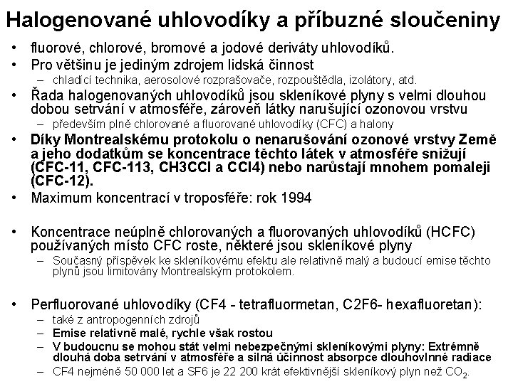
Halogenované uhlovodíky a příbuzné sloučeniny • fluorové, chlorové, bromové a jodové deriváty uhlovodíků. • Pro většinu je jediným zdrojem lidská činnost – chladící technika, aerosolové rozprašovače, rozpouštědla, izolátory, atd. • Řada halogenovaných uhlovodíků jsou skleníkové plyny s velmi dlouhou dobou setrvání v atmosféře, zároveň látky narušující ozonovou vrstvu – především plně chlorované a fluorované uhlovodíky (CFC) a halony • Díky Montrealskému protokolu o nenarušování ozonové vrstvy Země a jeho dodatkům se koncentrace těchto látek v atmosféře snižují (CFC-11, CFC-113, CH 3 CCl a CCl 4) nebo narůstají mnohem pomaleji (CFC-12). • Maximum koncentrací v troposféře: rok 1994 • Koncentrace neúplně chlorovaných a fluorovaných uhlovodíků (HCFC) používaných místo CFC roste, některé jsou skleníkové plyny – Současný příspěvek ke skleníkovému efektu ale relativně malý a budoucí emise těchto plynů jsou limitovány Montrealským protokolem. • Perfluorované uhlovodíky (CF 4 - tetrafluormetan, C 2 F 6 - hexafluoretan): – také z antropogenních zdrojů – Emise relativně malé, rychle však rostou – V budoucnu se mohou stát velmi nebezpečnými skleníkovými plyny: Extrémně dlouhá doba setrvání v atmosféře a silná účinnost absorpce dlouhovlnné radiace – CF 4 nejméně 50 000 let a SF 6 je 22 200 krát efektivnější skleníkový plyn než CO 2.

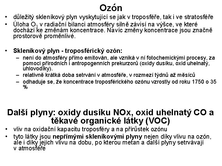
Ozón • důležitý skleníkový plyn vyskytující se jak v troposféře, tak i ve stratosféře • Úloha O 3 v radiační bilanci atmosféry silně závisí na výšce, ve které dochází ke změnám koncentrace. Navíc změny koncentrace jsou značně prostorově proměnlivé. • Skleníkový plyn - troposférický ozón: – není do atmosféry přímo emitován, ale vzniká v ní fotochemickými procesy, za pomoci přírodních i antropogenních prekurzorů (oxidy dusíku, oxid uhelnatý, uhlovodíky). – relativně krátká doba setrvání v atmosféře, v rozmezí týdnů až měsíců – odhaduje se, že koncentrace troposférického ozónu vzrostly od roku 1750 o 35 % Další plyny: oxidy dusíku NOx, oxid uhelnatý CO a těkavé organické látky (VOC) • vliv na oxidační kapacitu troposféry a na přírůstek ozónu • tyto látky jsou nepřímými skleníkovými plyny nejen díky vlivu na ozón, ale i díky jejich vlivu na dobu, po kterou metan a další plyny setrvávají v atmosféře

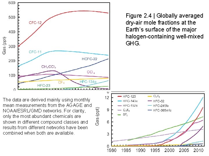
Figure 2. 4 | Globally averaged dry-air mole fractions at the Earth’s surface of the major halogen-containing well-mixed GHG. The data are derived mainly using monthly mean measurements from the AGAGE and NOAA/ESRL/GMD networks. For clarity, only the most abundant chemicals are shown in different compound classes and results from different networks have been combined when both are available.

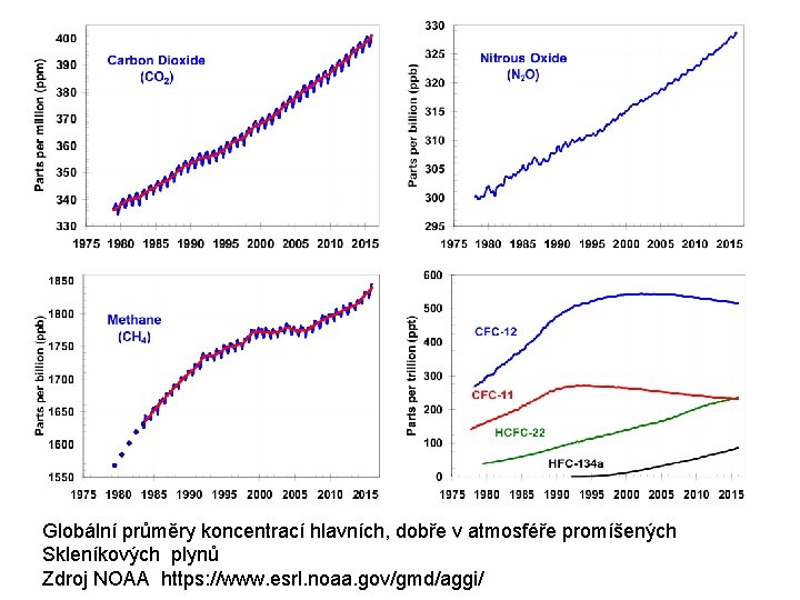
Globální průměry koncentrací hlavních, dobře v atmosféře promíšených Skleníkových plynů Zdroj NOAA https: //www. esrl. noaa. gov/gmd/aggi/

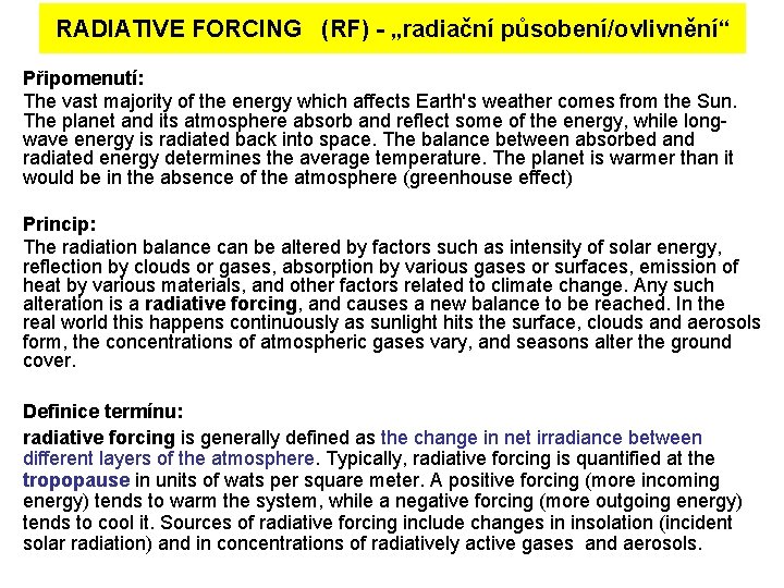
RADIATIVE FORCING (RF) - „radiační působení/ovlivnění“ Připomenutí: The vast majority of the energy which affects Earth's weather comes from the Sun. The planet and its atmosphere absorb and reflect some of the energy, while longwave energy is radiated back into space. The balance between absorbed and radiated energy determines the average temperature. The planet is warmer than it would be in the absence of the atmosphere (greenhouse effect) Princip: The radiation balance can be altered by factors such as intensity of solar energy, reflection by clouds or gases, absorption by various gases or surfaces, emission of heat by various materials, and other factors related to climate change. Any such alteration is a radiative forcing, and causes a new balance to be reached. In the real world this happens continuously as sunlight hits the surface, clouds and aerosols form, the concentrations of atmospheric gases vary, and seasons alter the ground cover. Definice termínu: radiative forcing is generally defined as the change in net irradiance between different layers of the atmosphere. Typically, radiative forcing is quantified at the tropopause in units of wats per square meter. A positive forcing (more incoming energy) tends to warm the system, while a negative forcing (more outgoing energy) tends to cool it. Sources of radiative forcing include changes in insolation (incident solar radiation) and in concentrations of radiatively active gases and aerosols.

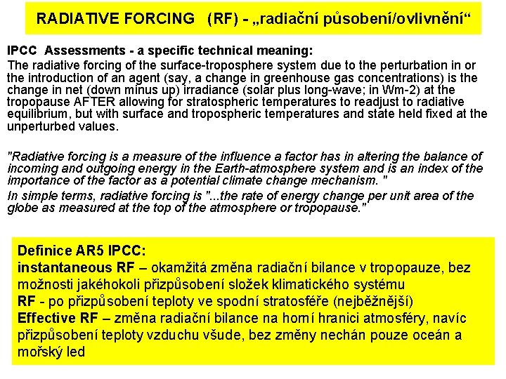
RADIATIVE FORCING (RF) - „radiační působení/ovlivnění“ IPCC Assessments - a specific technical meaning: The radiative forcing of the surface-troposphere system due to the perturbation in or the introduction of an agent (say, a change in greenhouse gas concentrations) is the change in net (down minus up) irradiance (solar plus long-wave; in Wm-2) at the tropopause AFTER allowing for stratospheric temperatures to readjust to radiative equilibrium, but with surface and tropospheric temperatures and state held fixed at the unperturbed values. "Radiative forcing is a measure of the influence a factor has in altering the balance of incoming and outgoing energy in the Earth-atmosphere system and is an index of the importance of the factor as a potential climate change mechanism. " In simple terms, radiative forcing is ". . . the rate of energy change per unit area of the globe as measured at the top of the atmosphere or tropopause. " Definice AR 5 IPCC: instantaneous RF – okamžitá změna radiační bilance v tropopauze, bez možnosti jakéhokoli přizpůsobení složek klimatického systému RF - po přizpůsobení teploty ve spodní stratosféře (nejběžnější) Effective RF – změna radiační bilance na horní hranici atmosféry, navíc přizpůsobení teploty vzduchu všude, bez změny nechán pouze oceán a mořský led

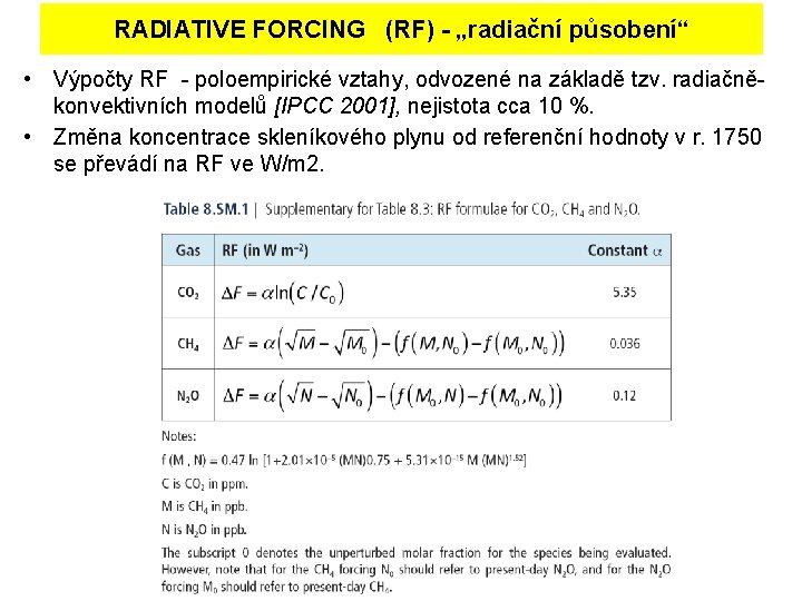
RADIATIVE FORCING (RF) - „radiační působení“ • Výpočty RF - poloempirické vztahy, odvozené na základě tzv. radiačněkonvektivních modelů [IPCC 2001], nejistota cca 10 %. • Změna koncentrace skleníkového plynu od referenční hodnoty v r. 1750 se převádí na RF ve W/m 2.

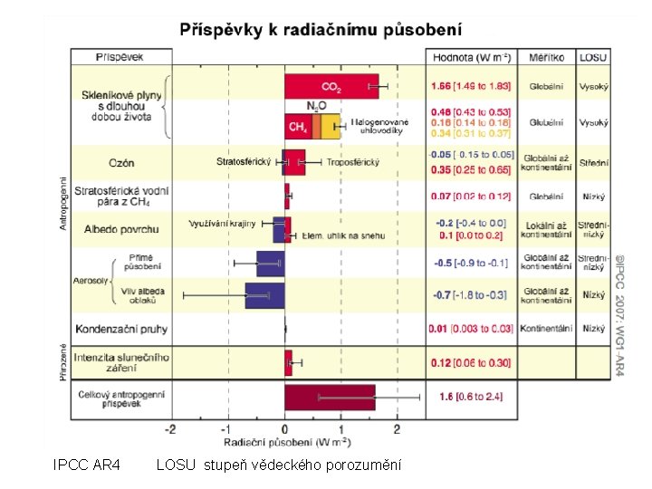
IPCC AR 4 LOSU stupeň vědeckého porozumění

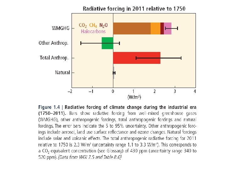
Global Warming Potential (GWP) GWP is a relative measure of how much heat a greenhouse gas traps in the atmosphere. It compares the amount of heat trapped by a certain mass of the gas in question to the amount of heat trapped by a similar mass of carbon dioxide. It is the time-integrated RF due to a pulse emission of a given component, relative to a pulse emission of an equal mass of CO 2. A GWP is calculated over a specific time interval, commonly 20, 100 or 500 years. GWP is expressed as a factor of carbon dioxide (whose GWP is standardized to 1). For example, the 20 years GWP of methane is 72, which means that if the same mass of methane and carbon dioxide were introduced into the atmosphere, that methane will trap 72 times more heat than the carbon dioxide over the next 20 years. The GWP depends on the following factors: the absorption of infrared radiation by a given species, the spectral location of its absorbing wavelengths, the atmospheric lifetime of the species. Thus, a high GWP correlates with a large infrared absorption and a long atmospheric lifetime. The dependence of GWP on the wavelength of absorption is more complicated. Even if a gas absorbs radiation efficiently at a certain wavelength, this may not affect its GWP much if the atmosphere already absorbs most radiation at that wavelength. A gas has the most effect if it absorbs in a "window" of wavelengths where the atmosphere is fairly transparent. However, the GWP does not lead to equivalence with temperature or other climate variables. Thus, the name ‘Global Warming Potential’ may be somewhat misleading, and ‘relative cumulative forcing index’ would be more appropriate.

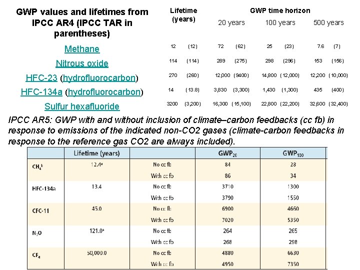
GWP values and lifetimes from IPCC AR 4 (IPCC TAR in parentheses) Lifetime (years) Methane GWP time horizon 20 years 100 years 500 years 12 (12) 72 (62) 25 (23) 7. 6 (7) Nitrous oxide 114 (114) 289 (275) 298 (296) 153 (156) HFC-23 (hydrofluorocarbon) 270 (260) 12, 000 (9400) 14, 800 (12, 000) 12, 200 (10, 000) HFC-134 a (hydrofluorocarbon) 14 (13. 8) 3, 830 (3, 300) 1, 430 (1, 300) 435 (400) 3200 (3, 200) 16, 300 (15, 100) 22, 800 (22, 200) 32, 600 (32, 400) Sulfur hexafluoride IPCC AR 5: GWP with and without inclusion of climate–carbon feedbacks (cc fb) in response to emissions of the indicated non-CO 2 gases (climate-carbon feedbacks in response to the reference gas CO 2 are always included).

Radiační působení skleníkových plynů

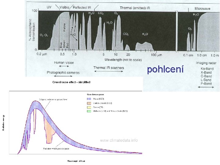
pohlcení

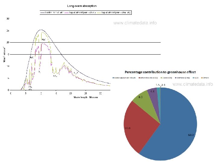
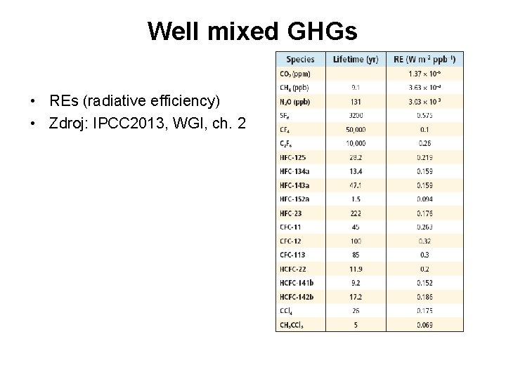
Well mixed GHGs • REs (radiative efficiency) • Zdroj: IPCC 2013, WGI, ch. 2

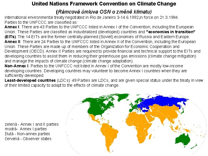
United Nations Framework Convention on Climate Change (Rámcová úmluva OSN o změně klimatu) international environmental treaty negotiated in Rio de Janeiro 3 -14. 6. 1992, in force on 21. 3. 1994. Parties to the UNFCCC are classified as: Annex I: There are 43 Parties to the UNFCCC listed in Annex I of the Convention, including the European Union. These Parties are classified as industrialized (developed) countries and "economies in transition" (EITs). The 14 EITs are the former centrally-planned (Soviet) economies of Russia and Eastern Europe. Annex II: There are 24 Parties to the UNFCCC listed in Annex II of the Convention, including the European Union. These Parties are made up of members of the Organization for Economic Cooperation and Development (OECD). Annex II Parties are required to provide financial and technical support to the EITs and developing countries to assist them in reducing their greenhouse gas emissions (climate change mitigation) and manage the impacts of climate change (climate change adaptation). Non-Annex I: Parties to the UNFCCC not listed in Annex I of the Convention are mostly low-income developing countries. Developing countries may volunteer to become Annex I countries when they are sufficiently developed. Least-developed countries (LDCs): 49 Parties are LDCs, and are given special status under the treaty in view of their limited capacity to adapt to the effects of climate change. zelená - Annex I and II parties modrá- Annex I parties žlutá - Non-annex parties červená - Observer states

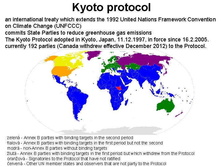
Kyoto protocol an international treaty which extends the 1992 United Nations Framework Convention on Climate Change (UNFCCC) commits State Parties to reduce greenhouse gas emissions The Kyoto Protocol adopted in Kyoto, Japan, 11. 12. 1997, in force since 16. 2. 2005. currently 192 parties (Canada withdrew effective December 2012) to the Protocol. zelená - Annex B parties with binding targets in the second period fialová - Annex B parties with binding targets in the first period but not the second modrá - non-Annex B parties without binding targets žlutá - Annex B parties with binding targets in the first period but which withdrew from the Protocol oranžová - Signatories to the Protocol that have not ratified červená - Other UN member states and observers that are not party to the Protocol

Global Carbon Budget web projektu: http: //www. globalcarbonproject. org/carbonbudget/ prezentace a infografika: http: //www. globalcarbonproject. org/carbonbudget/16/presentation. htm studie, analýza, popis metodiky http: //www. earth-syst-sci-data. net/8/605/2016/ Global carbon atlas http: //www. globalcarbonatlas. org/ Následují vybrané slidy a informace

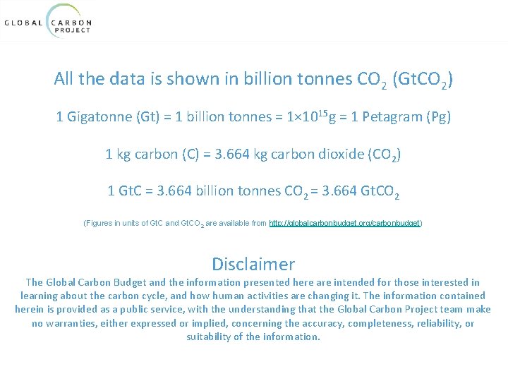
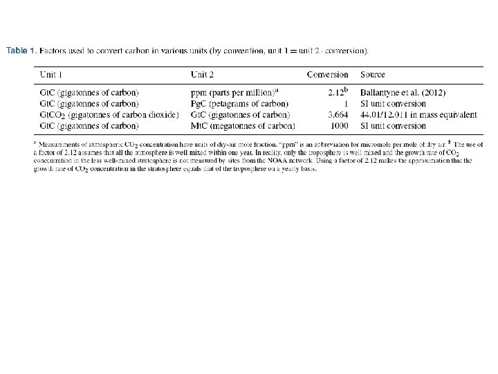
All the data is shown in billion tonnes CO 2 (Gt. CO 2) 1 Gigatonne (Gt) = 1 billion tonnes = 1× 1015 g = 1 Petagram (Pg) 1 kg carbon (C) = 3. 664 kg carbon dioxide (CO 2) 1 Gt. C = 3. 664 billion tonnes CO 2 = 3. 664 Gt. CO 2 (Figures in units of Gt. C and Gt. CO 2 are available from http: //globalcarbonbudget. org/carbonbudget) Disclaimer The Global Carbon Budget and the information presented here are intended for those interested in learning about the carbon cycle, and how human activities are changing it. The information contained herein is provided as a public service, with the understanding that the Global Carbon Project team make no warranties, either expressed or implied, concerning the accuracy, completeness, reliability, or suitability of the information.

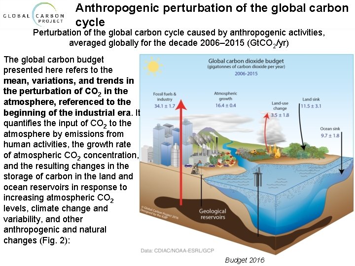
Anthropogenic perturbation of the global carbon cycle Perturbation of the global carbon cycle caused by anthropogenic activities, averaged globally for the decade 2006– 2015 (Gt. CO 2/yr) The global carbon budget presented here refers to the mean, variations, and trends in the perturbation of CO 2 in the atmosphere, referenced to the beginning of the industrial era. It quantifies the input of CO 2 to the atmosphere by emissions from human activities, the growth rate of atmospheric CO 2 concentration, and the resulting changes in the storage of carbon in the land ocean reservoirs in response to increasing atmospheric CO 2 levels, climate change and variability, and other anthropogenic and natural changes (Fig. 2): Source: CDIAC; NOAA-ESRL; Le Quéré et al 2016; Global Carbon Budget 2016

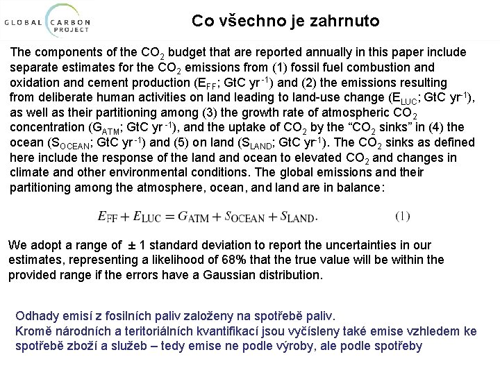
Co všechno je zahrnuto The components of the CO 2 budget that are reported annually in this paper include separate estimates for the CO 2 emissions from (1) fossil fuel combustion and oxidation and cement production (EFF; Gt. C yr -1) and (2) the emissions resulting from deliberate human activities on land leading to land-use change (ELUC; Gt. C yr-1), as well as their partitioning among (3) the growth rate of atmospheric CO 2 concentration (GATM; Gt. C yr -1), and the uptake of CO 2 by the “CO 2 sinks” in (4) the ocean (SOCEAN; Gt. C yr -1) and (5) on land (SLAND; Gt. C yr-1). The CO 2 sinks as defined here include the response of the land ocean to elevated CO 2 and changes in climate and other environmental conditions. The global emissions and their partitioning among the atmosphere, ocean, and land are in balance: We adopt a range of ± 1 standard deviation to report the uncertainties in our estimates, representing a likelihood of 68% that the true value will be within the provided range if the errors have a Gaussian distribution. Odhady emisí z fosilních paliv založeny na spotřebě paliv. Kromě národních a teritoriálních kvantifikací jsou vyčísleny také emise vzhledem ke spotřebě zboží a služeb – tedy emise ne podle výroby, ale podle spotřeby

Co všechno je zahrnuto - EFF Odhady emisí z fosilních paliv založeny na spotřebě paliv. Kromě národních a teritoriálních kvantifikací jsou vyčísleny také emise vzhledem ke spotřebě zboží a služeb – tedy emise ne podle výroby, ale podle spotřeby National emission inventories take a territorial (production) perspective and “include greenhouse gas emissions and removals taking place within national territory and offshore areas over which the country has jurisdiction” (Rypdal et al. , 2006). That is, emissions are allocated to the country where and when the emissions actually occur. The territorial emission inventory of an individual country does not include the emissions from the production of goods and services produced in other countries (e. g. food and clothes) that are used for consumption. Consumption-based emission inventories for an individual country are another attribution point of view that allocates global emissions to products that are consumed within a country; these inventories are conceptually calculated as the territorial emissions minus the “embedded” territorial emissions to produce exported products plus the emissions in other countries to produce imported products: consumption = territorial – exports + imports The difference between the territorial- and consumption-based emission inventories is the net transfer (exports minus imports) of emissions from the production of internationally traded products. Consumption-based emission attribution results (e. g. Davis and Caldeira, 2010) provide additional information to territorial-based emissions that can be used to understand emission drivers (Hertwich and Peters, 2009), quantify emission transfers by the trade of products between countries (Peters et al. , 2011 b), and potentially design more effective andefficient climate policy (Peters and Hertwich, 2008).

Co všechno je zahrnuto - ELUC Land-use-change emissions reported here (ELUC) include CO 2 fluxes from deforestation, afforestation, logging (forest degradation and harvest activity), shifting cultivation (cycle of cutting forest for agriculture and then abandoning), and regrowth of forests following wood harvest or abandonment of agriculture. Only some land management activities are included in our land-use-change emissions estimates. Some of these activities lead to emissions of CO 2 to the atmosphere, while others lead to CO 2 sinks. ELUC is the net sum of all anthropogenic activities considered. Our annual estimate for 1959– 2010 is primarily based on net forest area change and biomass data from the Forest Resource Assessment (FRA) of the Food and Agriculture Organization (FAO), which are only available at intervals of 5 years. We use FAO FRA 2010 here (Houghton et al. , 2012) and present preliminary results of an update using the FAO FRA 2015 (Houghton and Nassikas, 2016). Interannual variability in emissions due to deforestation and degradation have been coarsely estimated from satellite-based fire activity in tropical forest areas (Sect. 2. 2. 2; Giglio et al. , 2013; van der Werf et al. , 2010). Land-use-change CO 2 emissions have been estimated using an ensemble of Dynamic global vegetation models (DGVMs) simulations. Two sets of simulations were performed with the DGVMs, first forced with historical changes in land-cover distribution, climate, atmospheric CO 2 concentration, and N deposition, and second, as further described below with a time-invariant pre-industrial land-cover distribution, allowing for estimation of, by difference with the first simulation, the dynamic evolution of biomass and soil carbon pools in response to prescribed landcover change.

Co všechno je zahrnuto Ocean CO 2 sink – odhad založen na kombinaci pozorování a modelových výsledků Růst koncentrací v atmosféře – pozorování, nejdříve Mauna Loa, později globální průměr (od roku 1980) Terrestrial CO 2 sink - The difference between, on the one hand, fossil fuel (EFF) and land-usechange emissions (ELUC) and, on the other hand, the growth rate in atmospheric CO 2 concentration (GATM) and the ocean CO 2 sink (SOCEAN) is attributable to the net sink of CO 2 in terrestrial vegetation and soils (SLAND), within the given uncertainties (Eq. 1). Thus, this sink can be estimated as the residual of the other terms in the mass balance budget, as well as directly calculated using DGVMs. The residual land sink (SLAND) is thought to be in part because of the fertilising effect of rising atmospheric CO 2 on plant growth, N deposition, and effects of climate change such as the lengthening of the growing season in northern temperate and boreal areas. SLAND does not include gross land sinks directly resulting from land-use change (e. g. regrowth of vegetation) as these are estimated as part of the net land-use flux (ELUC). System boundaries make it difficult to exactly attribute CO 2 fluxes on land between SLAND and ELUC (Erb et al. , 2013), and by design most of the uncertainties in our method are allocated to SLAND for those processes that are poorly known or represented in models.

Prezentace Global Carbon Budget výběr slidů

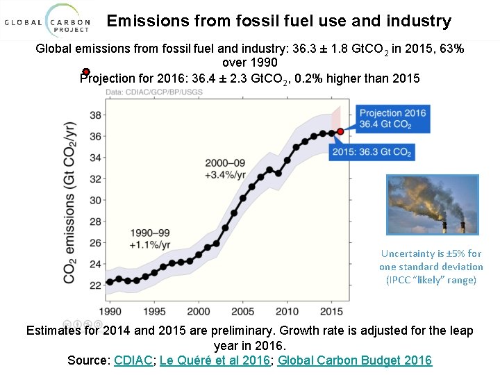
Emissions from fossil fuel use and industry Global emissions from fossil fuel and industry: 36. 3 ± 1. 8 Gt. CO 2 in 2015, 63% over 1990 Projection for 2016: 36. 4 ± 2. 3 Gt. CO 2, 0. 2% higher than 2015 Uncertainty is ± 5% for one standard deviation (IPCC “likely” range) Estimates for 2014 and 2015 are preliminary. Growth rate is adjusted for the leap year in 2016. Source: CDIAC; Le Quéré et al 2016; Global Carbon Budget 2016

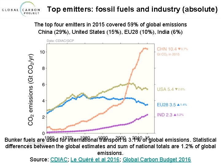
Top emitters: fossil fuels and industry (absolute) The top four emitters in 2015 covered 59% of global emissions China (29%), United States (15%), EU 28 (10%), India (6%) Bunker fuels are used for international transport is 3. 1% of global emissions. Statistical differences between the global estimates and sum of national totals are 1. 2% of global emissions. Source: CDIAC; Le Quéré et al 2016; Global Carbon Budget 2016

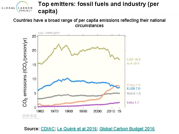
Top emitters: fossil fuels and industry (per capita) Countries have a broad range of per capita emissions reflecting their national circumstances Source: CDIAC; Le Quéré et al 2016; Global Carbon Budget 2016

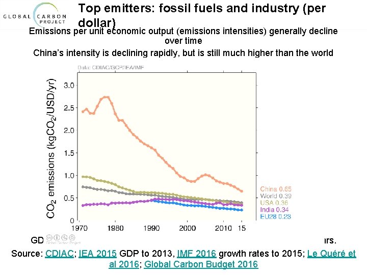
Top emitters: fossil fuels and industry (per dollar) Emissions per unit economic output (emissions intensities) generally decline over time China’s intensity is declining rapidly, but is still much higher than the world average GDP are measured in purchasing power parity (PPP) terms in 2005 dollars. Source: CDIAC; IEA 2015 GDP to 2013, IMF 2016 growth rates to 2015; Le Quéré et al 2016; Global Carbon Budget 2016

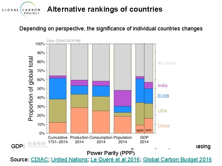
Alternative rankings of countries Depending on perspective, the significance of individual countries changes GDP: Gross Domestic Product in Market Exchange Rates (MER) and Purchasing Power Parity (PPP) Source: CDIAC; United Nations; Le Quéré et al 2016; Global Carbon Budget 2016

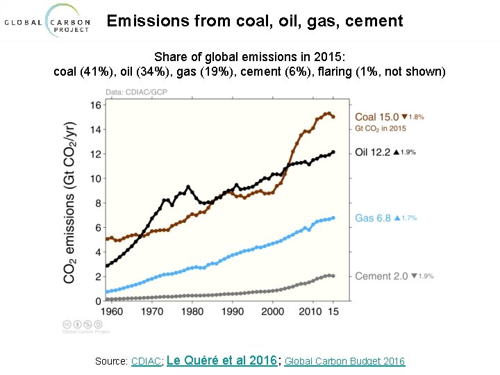
Emissions from coal, oil, gas, cement Share of global emissions in 2015: coal (41%), oil (34%), gas (19%), cement (6%), flaring (1%, not shown) Source: CDIAC; Le Quéré et al 2016; Global Carbon Budget 2016

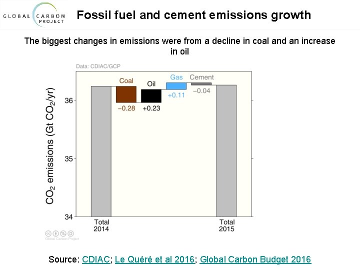
Fossil fuel and cement emissions growth The biggest changes in emissions were from a decline in coal and an increase in oil Source: CDIAC; Le Quéré et al 2016; Global Carbon Budget 2016

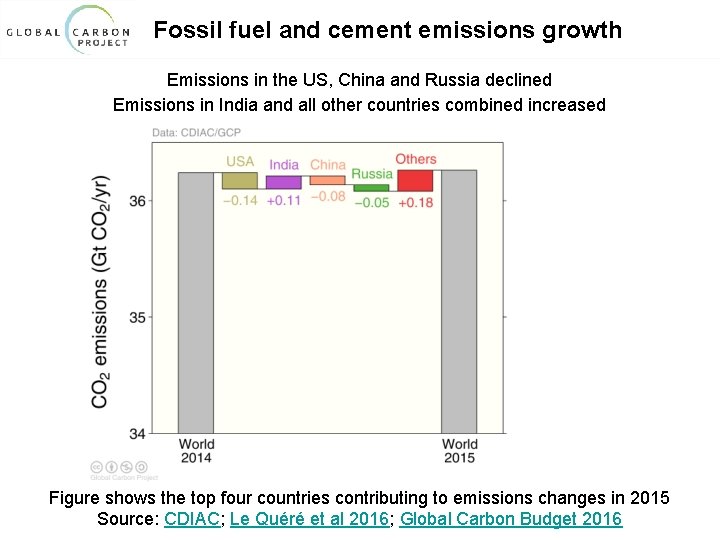
Fossil fuel and cement emissions growth Emissions in the US, China and Russia declined Emissions in India and all other countries combined increased Figure shows the top four countries contributing to emissions changes in 2015 Source: CDIAC; Le Quéré et al 2016; Global Carbon Budget 2016

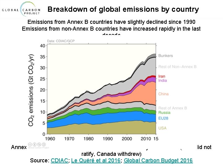
Breakdown of global emissions by country Emissions from Annex B countries have slightly declined since 1990 Emissions from non-Annex B countries have increased rapidly in the last decade Annex B countries had emission commitments in the Kyoto Protocol (USA did not ratify, Canada withdrew) Source: CDIAC; Le Quéré et al 2016; Global Carbon Budget 2016

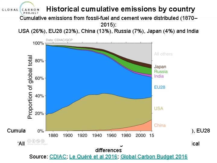
Historical cumulative emissions by country Cumulative emissions from fossil-fuel and cement were distributed (1870– 2015): USA (26%), EU 28 (23%), China (13%), Russia (7%), Japan (4%) and India (3%) Cumulative emissions (1990– 2015) were distributed China (21%), USA (20%), EU 28 (14%), Russia (6%), India/Japan (4%) ‘All others’ includes all other countries along with bunker fuels and statistical differences Source: CDIAC; Le Quéré et al 2016; Global Carbon Budget 2016

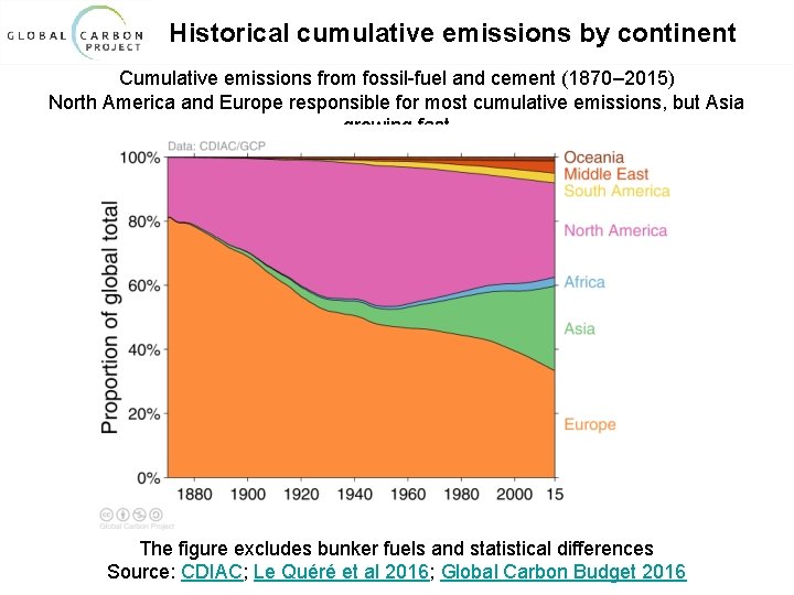
Historical cumulative emissions by continent Cumulative emissions from fossil-fuel and cement (1870– 2015) North America and Europe responsible for most cumulative emissions, but Asia growing fast The figure excludes bunker fuels and statistical differences Source: CDIAC; Le Quéré et al 2016; Global Carbon Budget 2016

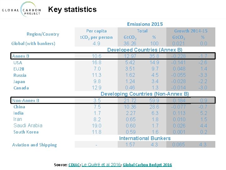
Key statistics Emissions 2015 Region/Country Global (with bunkers) Annex B USA EU 28 Russia Japan Canada Non-Annex B China India Iran Saudi Arabia South Korea Aviation and Shipping Per capita Total Growth 2014 -15 t. CO 2 person Gt. CO 2 % 4. 9 36. 26 100 0. 021 0. 0 Developed Countries (Annex B) 10. 6 12. 97 35. 8 -0. 228 -1. 7 16. 8 5. 42 14. 9 -0. 141 -2. 6 7. 0 3. 51 9. 7 0. 048 1. 4 11. 3 1. 62 4. 5 -0. 055 -3. 3 9. 8 1. 24 3. 4 -0. 028 -2. 2 12. 9 0. 46 1. 3 -0. 014 -3. 0 Developing Countries (Non-Annex B) 3. 5 21. 72 59. 9 0. 184 0. 9 7. 5 10. 36 28. 6 -0. 077 -0. 7 1. 7 2. 27 6. 3 0. 113 5. 2 8. 2 0. 65 1. 8 0. 010 1. 5 19. 0 0. 60 1. 7 0. 026 4. 4 11. 8 0. 59 1. 6 0. 001 0. 2 International Bunkers 1. 57 4. 3 0. 065 4. 3 Source: CDIAC; Le Quéré et al 2016; Global Carbon Budget 2016

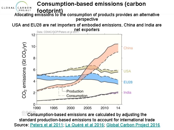
Consumption-based emissions (carbon footprint) Allocating emissions to the consumption of products provides an alternative perspective USA and EU 28 are net importers of embodied emissions, China and India are net exporters Consumption-based emissions are calculated by adjusting the standard production-based emissions to account for international trade Source: Peters et al 2011; Le Quéré et al 2016; Global Carbon Project 2016

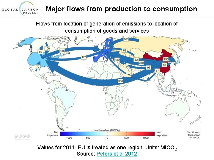
Major flows from production to consumption Flows from location of generation of emissions to location of consumption of goods and services Values for 2011. EU is treated as one region. Units: Mt. CO 2 Source: Peters et al 2012

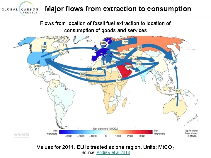
Major flows from extraction to consumption Flows from location of fossil fuel extraction to location of consumption of goods and services Values for 2011. EU is treated as one region. Units: Mt. CO 2 Source: Andrew et al 2013

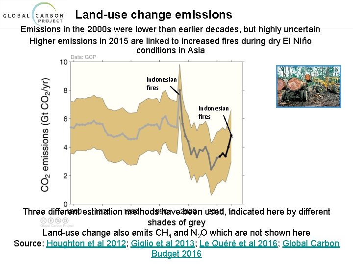
Land-use change emissions Emissions in the 2000 s were lower than earlier decades, but highly uncertain Higher emissions in 2015 are linked to increased fires during dry El Niño conditions in Asia Indonesian fires Three different estimation methods have been used, indicated here by different shades of grey Land-use change also emits CH 4 and N 2 O which are not shown here Source: Houghton et al 2012; Giglio et al 2013; Le Quéré et al 2016; Global Carbon Budget 2016

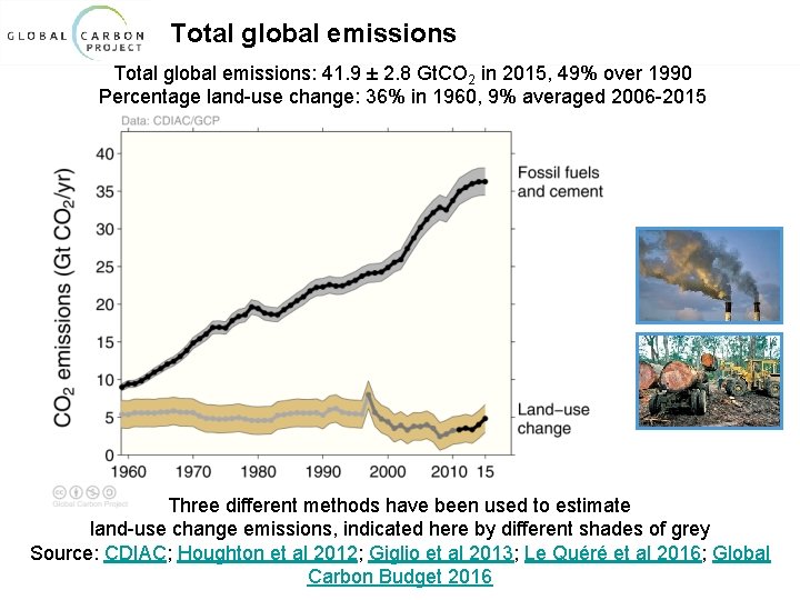
Total global emissions: 41. 9 ± 2. 8 Gt. CO 2 in 2015, 49% over 1990 Percentage land-use change: 36% in 1960, 9% averaged 2006 -2015 Three different methods have been used to estimate land-use change emissions, indicated here by different shades of grey Source: CDIAC; Houghton et al 2012; Giglio et al 2013; Le Quéré et al 2016; Global Carbon Budget 2016

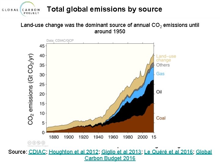
Total global emissions by source Land-use change was the dominant source of annual CO 2 emissions until around 1950 Others: Emissions from cement production and gas flaring Source: CDIAC; Houghton et al 2012; Giglio et al 2013; Le Quéré et al 2016; Global Carbon Budget 2016

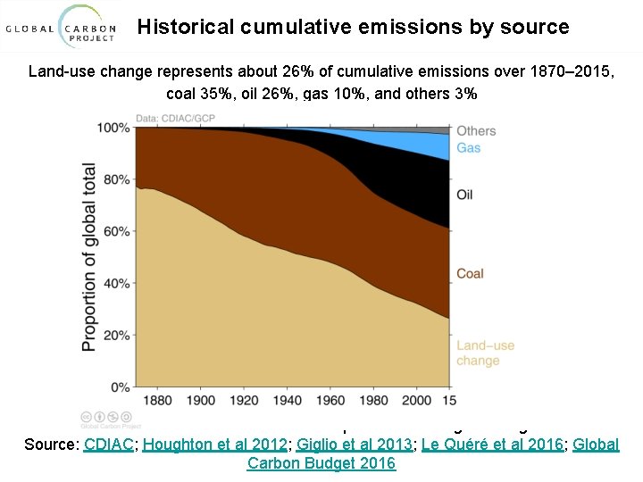
Historical cumulative emissions by source Land-use change represents about 26% of cumulative emissions over 1870– 2015, coal 35%, oil 26%, gas 10%, and others 3% Others: Emissions from cement production and gas flaring Source: CDIAC; Houghton et al 2012; Giglio et al 2013; Le Quéré et al 2016; Global Carbon Budget 2016

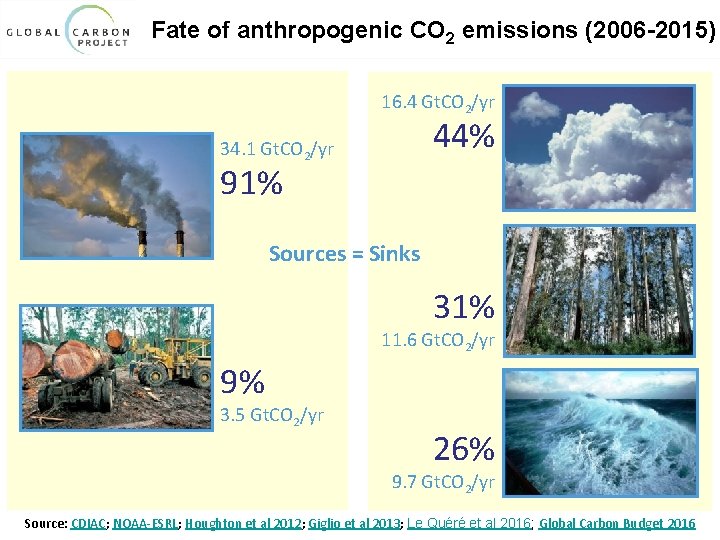
Fate of anthropogenic CO 2 emissions (2006 -2015) 16. 4 Gt. CO 2/yr 44% 34. 1 Gt. CO 2/yr 91% Sources = Sinks 31% 11. 6 Gt. CO 2/yr 9% 3. 5 Gt. CO 2/yr 26% 9. 7 Gt. CO 2/yr Source: CDIAC; NOAA-ESRL; Houghton et al 2012; Giglio et al 2013; Le Quéré et al 2016; Global Carbon Budget 2016

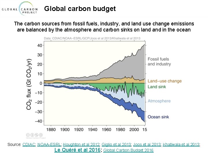
Global carbon budget The carbon sources from fossil fuels, industry, and land use change emissions are balanced by the atmosphere and carbon sinks on land in the ocean Source: CDIAC; NOAA-ESRL; Houghton et al 2012; Giglio et al 2013; Joos et al 2013; Khatiwala et al 2013; Le Quéré et al 2016; Global Carbon Budget 2016

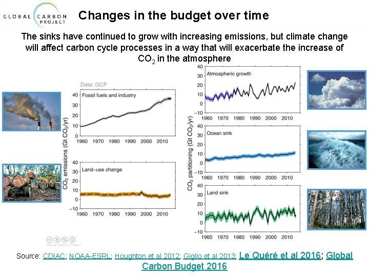
Changes in the budget over time The sinks have continued to grow with increasing emissions, but climate change will affect carbon cycle processes in a way that will exacerbate the increase of CO 2 in the atmosphere Source: CDIAC; NOAA-ESRL; Houghton et al 2012; Giglio et al 2013; Le Quéré et al 2016; Global Carbon Budget 2016

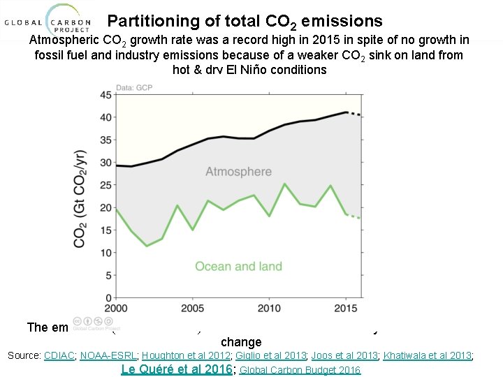
Partitioning of total CO 2 emissions Atmospheric CO 2 growth rate was a record high in 2015 in spite of no growth in fossil fuel and industry emissions because of a weaker CO 2 sink on land from hot & dry El Niño conditions The emissions (shown in black) include fossil fuels and industry and land-use change Source: CDIAC; NOAA-ESRL; Houghton et al 2012; Giglio et al 2013; Joos et al 2013; Khatiwala et al 2013; Le Quéré et al 2016; Global Carbon Budget 2016

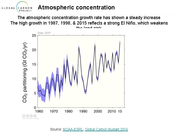
Atmospheric concentration The atmospheric concentration growth rate has shown a steady increase The high growth in 1987, 1998, & 2015 reflects a strong El Niño, which weakens the land sink Source: NOAA-ESRL; Global Carbon Budget 2016

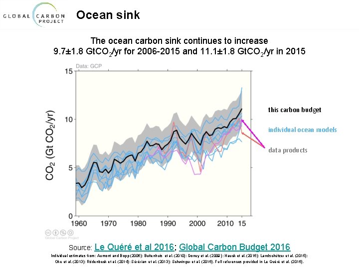
Ocean sink The ocean carbon sink continues to increase 9. 7± 1. 8 Gt. CO 2/yr for 2006 -2015 and 11. 1± 1. 8 Gt. CO 2/yr in 2015 this carbon budget individual ocean models data products Source: Le Quéré et al 2016; Global Carbon Budget 2016 Individual estimates from: Aumont and Bopp (2006); Buitenhuis et al. (2010); Doney et al. (2009 ); Hauck et al. (2016); Landschützer et al. (2015); Oke et al. (2013); Rödenbeck et al. (2014); Sérérian et al. (2013); Schwinger et al. (2016). Full references provided in Le Quéré et al. (2016).

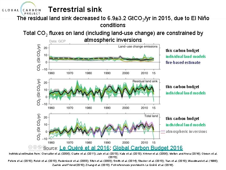
Terrestrial sink The residual land sink decreased to 6. 9± 3. 2 Gt. CO 2/yr in 2015, due to El Niño conditions Total CO 2 fluxes on land (including land-use change) are constrained by atmospheric inversions this carbon budget individual land models fire-based estimate this carbon budget individual land models atmospheric inversions Source: Le Quéré et al 2016; Global Carbon Budget 2016 Individual estimates from: Chevallier et al. (2005); Clarke et al. (2011); Jain et al. (2013); Kato et al. (2013); Krinner et al. (2005); Melton and Arora (2016); Oleson et al. (2013); Peters et al. (2010); Reick et al. (2013); Rodenbeck et al. (2003); Sitch et al. (2003); Smith et al. (2014); Stocker et al. (2013); Tian et al. (2010); Woodward et al. (1995); Zaehle and Friend (2010); Zhang et al. (2013). Full references provided in Le Quéré et al. (2016).

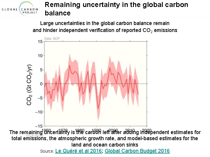
Remaining uncertainty in the global carbon balance Large uncertainties in the global carbon balance remain and hinder independent verification of reported CO 2 emissions The remaining uncertainty is the carbon left after adding independent estimates for total emissions, the atmospheric growth rate, and model-based estimates for the land ocean carbon sinks Source: Le Quéré et al 2016; Global Carbon Budget 2016

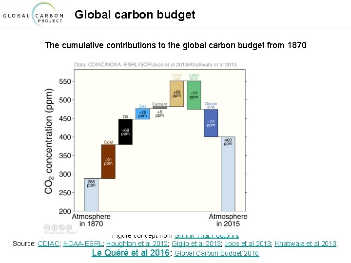
Global carbon budget The cumulative contributions to the global carbon budget from 1870 Figure concept from Shrink That Footprint Source: CDIAC; NOAA-ESRL; Houghton et al 2012; Giglio et al 2013; Joos et al 2013; Khatiwala et al 2013; Le Quéré et al 2016; Global Carbon Budget 2016

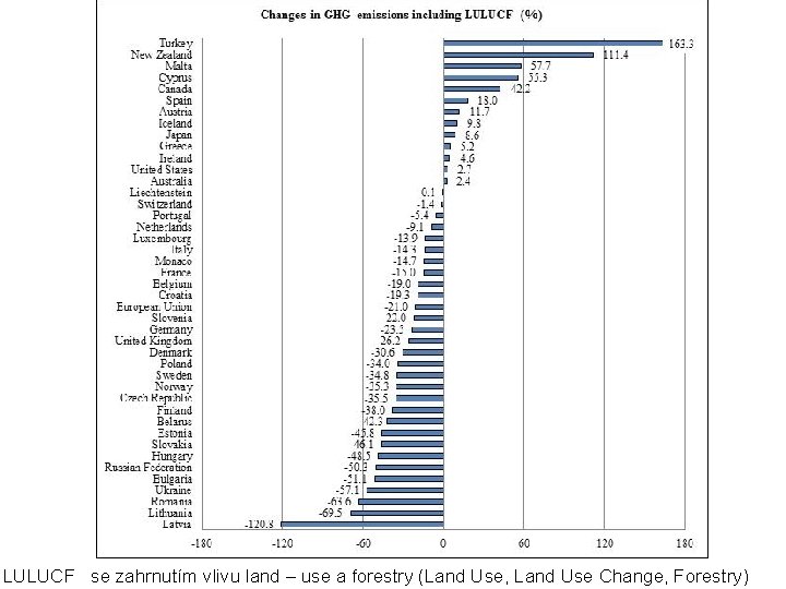
LULUCF se zahrnutím vlivu land – use a forestry (Land Use, Land Use Change, Forestry)

Scénáře změny klimatu a emisní scénáře Ø Projekce budoucího klimatu závisí také na mnoha faktorech ležících mimo oblast meteorologie a klimatologie. Ø Zkoumána je především závislost na emisích látek ovlivňujících radiační bilanci Země ( skleníkových plynů a aerosolů) -> emisní scénáře Ø Emise v budoucnosti jsou určovány vývojem lidské společnosti. Ø Dosud byly emisní scénáře založeny na odhadech možného ekonomického a populačního růstu, vývoje technologií atd. (tzv. socio-ekonomických scénářích) Ø Klimatické modely se pak užívají pro určování odezvy klimatického systému na určité scénáře emisí. Ø Vytvářejí se sady emisních scénářů založené na různých podmínkách budoucího vývoje společnosti - odhady neurčitostí projekcí budoucího klimatu Ø zahrnuty varianty vývoje směřujícího k vyrovnání rozdílů mezi bohatými a chudými zeměmi, i vývoje směřujícího k velmi heterogennímu světu.

Emisní scénáře Ø První sada emisních scénářů - IPCC roku 1990 (označována SA 90) - vyšetřovala 4 možné dráhy vývoje emisí. Ø scénáře IS 92 (IPCC 1992) - zahrnují velké množství sociálních a ekonomických podmínek - široké rozpětí možných emisí skleníkových plynů Ø Dosud byla většinou používána sada emisních scénářů tzv. SRES scénářů (Special Report on Emission Scenarios, IPCC 2000) Ø Nově se používají tzv. Representative concentration pathways (RCPs)

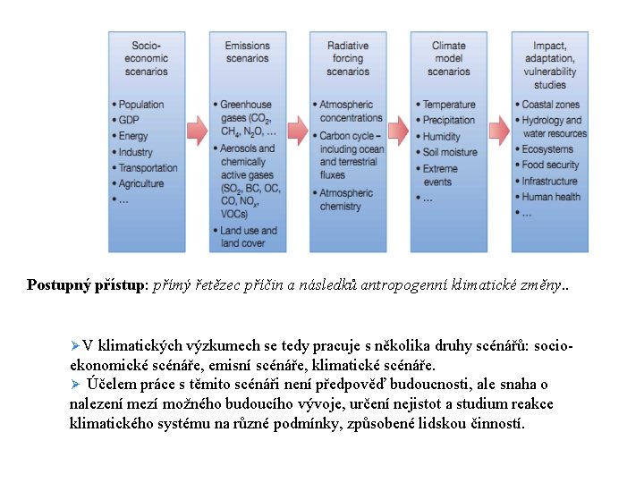
Postupný přístup: přímý řetězec příčin a následků antropogenní klimatické změny. . Ø V klimatických výzkumech se tedy pracuje s několika druhy scénářů: socio- ekonomické scénáře, emisní scénáře, klimatické scénáře. Ø Účelem práce s těmito scénáři není předpověď budoucnosti, ale snaha o nalezení mezí možného budoucího vývoje, určení nejistot a studium reakce klimatického systému na různé podmínky, způsobené lidskou činností.

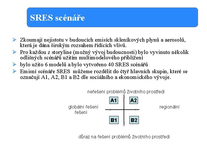
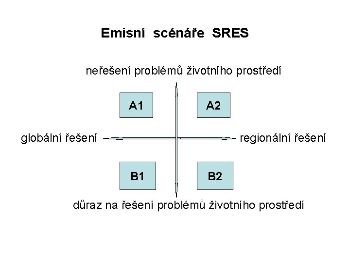
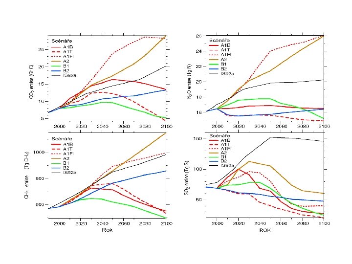
SRES scénáře Ø Zkoumají nejistotu v budoucích emisích skleníkových plynů a aerosolů, která je dána širokým rozsahem řídících vlivů. Ø Pro každou z storyline (možný vývoj budoucnosti) bylo vyvinuto několik odlišných scénářů užitím multimodelového přiblížení Ø bylo užito 6 modelů a bylo vytvořeno 40 SRES scénářů Ø Emisní scénáře SRES můžeme rozdělit do čtyř hlavních skupin, které se označují A 1, A 2, B 1 a B 2 dle sociálního a ekonomického vývoje. neřešení problémů životního prostředí A 1 A 2 globální řešení regionální řešení B 1 B 2 důraz na řešení problémů životního prostředí

Emisní scénáře SRES neřešení problémů životního prostředí A 1 A 2 globální řešení regionální řešení B 1 B 2 důraz na řešení problémů životního prostředí

SRES systém scénářů má čtyři hlavní „rodiny“ scénářů : A 1, A 2, B 1, B 2 Ø A 1 - svět s velmi rychlým růstem ekonomiky a vývojem nových technologií. Počet obyvatel Země dosáhne maxima v polovině příštího století a pak bude pomalu klesat. Tato rodina se dále dělí do tří skupin podle využívaných zdrojů energie: intenzivní využívání fosilní energie (A 1 FI), bez zdrojů fosilní energie (A 1 T) a rovnováha ve využívání všech druhů energie (A 1 B). Ø A 2 - velmi různorodý svět. Porodnost v různých regionech světa se daří stabilizovat velmi pomalu, tzn. populace stále roste až na 15 miliard v roce 2100. Ekonomický rozvoj je výrazně regionálně orientován, růst hrubého domácího produktu na jednoho obyvatele a technologické změny jsou pomalejší než u rodin A 1 nebo B 1. Základní ideou je spoléhat se sám na sebe a zachovat místní identitu, dodržovat místní tradice. Ø B 1 má v pozadí představu konvergentního, stmelujícího se světa, počet obyvatel na Zemi dosáhne svého maxima (8, 7 miliard) uprostřed 21. století a poté začne klesat na 7 miliard v roce 2100. Předpokládá se rychlý rozvoj informatiky, služeb, zavádění "čistých" účinných technologií. Důraz se klade na globální řešení ekonomických a sociálním problémů a ochranu životního prostředí, růst HDP "jde střední cestou". Ø B 2 - svět, ve kterém je kladen důraz na místní ekonomiku a trvale udržitelný rozvoj. Světová populace roste pomaleji než v A 2, pomalejší je i ekonomický rozvoj a změny v technologiích jsou různorodější než v A 1 a B 1.

Ø V každé rodině scénářů najdeme řadu variant, celkem se jedná o 40 scénářů, které zachycují široké spektrum demografických, ekonomických a technologických možností vývoje. Ø Žádná rodina scénářů není považována za více ani méně pravděpodobnou než ostatní. Ø Provádět odhady dopadů změny klimatu pro všech 40 SRES scénářů je velmi časově i finančně náročné. Proto byl pro rodiny scénářů A 2, B 1, B 2 zvolen ilustrativní zástupce, u první rodiny A 1 pak zástupci tři. Vznikla tak skupina šesti scénářů A 1 F 1, A 1 B, A 1 T, A 2, B 1, B 2, pro které byly přednostně počítány scénáře změny klimatu (u nás zejména A 1 B, A 2, B 1). Ø Bohužel i zdánlivě optimistický vývoj, kdy od poloviny století emise skleníkových plynů klesají, neznamená zastavení růstu koncentrací skleníkových plynů v atmosféře. Skleníkové plyny uvolněné do atmosféry zde zůstávají až několik desetiletí, pokles koncentrací se v tomto století nepředpokládá. Ø Podle téměř všech SRES scénářů (skupina 35 scénářů) radiační účinek CO 2, CH 4, N 2 O a troposférického ozónu stále poroste.

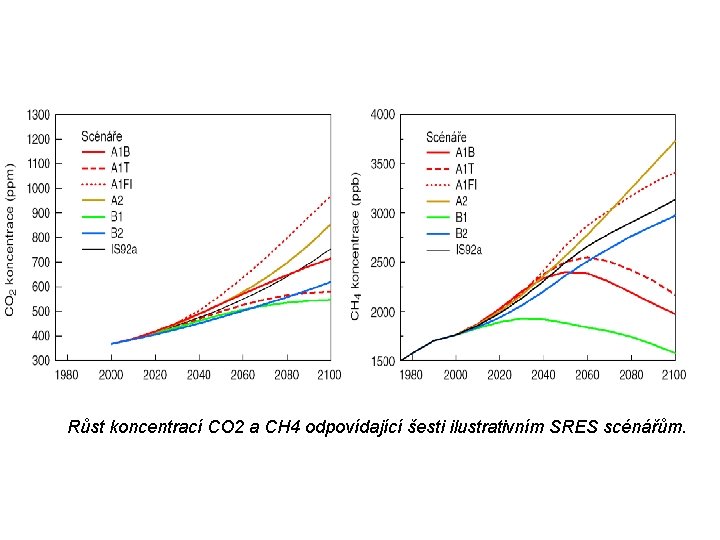
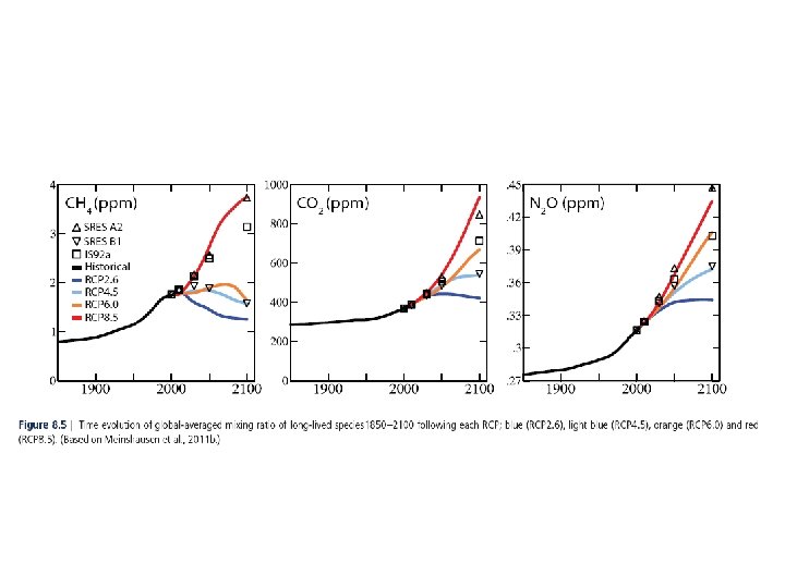
Růst koncentrací CO 2 a CH 4 odpovídající šesti ilustrativním SRES scénářům.

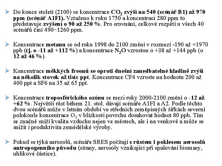
Ø Do konce století (2100) se koncentrace CO 2 zvýší na 540 (scénář B 1) až 970 ppm (scénář A 1 FI). Vztaženo k roku 1750 a koncentraci 280 ppm to představuje zvýšení o 90 až 250 %. Pro srovnání, celkové rozpětí u všech 40 scénářů činí 490− 1260 ppm. Ø Koncentrace metanu se od roku 1998 do 2100 změní v rozmezí -190 až +1970 ppb (tj. o -11 až +112 %) a koncentrace N 2 O vzrostou o +38 až +144 ppb (o 12 až 46 %). Ø Koncentrace měkkých freonů se oproti dnešní zanedbatelné hladině zvýší na několik stovek až tisíc ppt. Koncentrace CF 4 vzroste na hodnotu 200 až 400 ppt a SF 6 na 35 až 65 ppt. Ø Koncentrace troposférického ozónu se mezi roky 2000 -2100 změní o -12 až +62 %. Největší růst během 21. stol. dávají scénáře A 1 FI a A 2. Podle těchto dvou scénářů může v letním období ve středních zeměpisných šířkách severní polokoule koncentrace O 3 v blízkosti povrchu dosahovat hodnot 80 ppb. Tím se značně sníží kvalita vzduchu nejen ve městech, ale i na venkově a může se snížit i produktivita zemědělské výroby. Ø Pokud se týká aerosolů, scénáře SRES počítají s růstem i poklesem aerosolů antropogenního původu (sírany, aerosoly vznikající při spalování biomasy, uhlíkové částice).

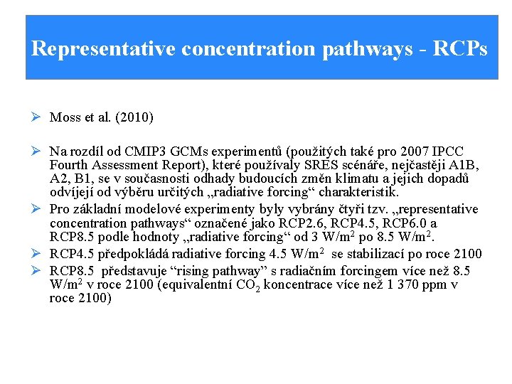
Representative concentration pathways - RCPs Ø Moss et al. (2010) Ø Na rozdíl od CMIP 3 GCMs experimentů (použitých také pro 2007 IPCC Fourth Assessment Report), které používaly SRES scénáře, nejčastěji A 1 B, A 2, B 1, se v současnosti odhady budoucích změn klimatu a jejich dopadů odvíjejí od výběru určitých „radiative forcing“ charakteristik. Ø Pro základní modelové experimenty byly vybrány čtyři tzv. „representative concentration pathways“ označené jako RCP 2. 6, RCP 4. 5, RCP 6. 0 a RCP 8. 5 podle hodnoty „radiative forcing“ od 3 W/m 2 po 8. 5 W/m 2. Ø RCP 4. 5 předpokládá radiative forcing 4. 5 W/m 2 se stabilizací po roce 2100 Ø RCP 8. 5 představuje “rising pathway” s radiačním forcingem více než 8. 5 W/m 2 v roce 2100 (equivalentní CO 2 koncentrace více než 1 370 ppm v roce 2100)

Representative Concentration Pathways (RCPs) Ø Nový přístup k vytváření scénářů klimatických změn Ø Nejdříve stanoveny 4 tzv. „reprezentativní dráhy koncentrací“ (RCPs) – tj. scénáře budoucího radiačního forcingu o tj. změna radiační bilance v troposféře způsobená změnou složek atmosféry (změnou koncentrací plynů v atmosféře např. CO 2) o ve zprávě IPCC AR 4 hodnoty radiačního forecingu pro změnu vzhledem k pre-industriálnímu období 1750 Ø Ø RCPs stanoveny z existující odborné literatury Poskytují potřebné vstupy emisí, koncentrací a využití půdy do klimatických modelů

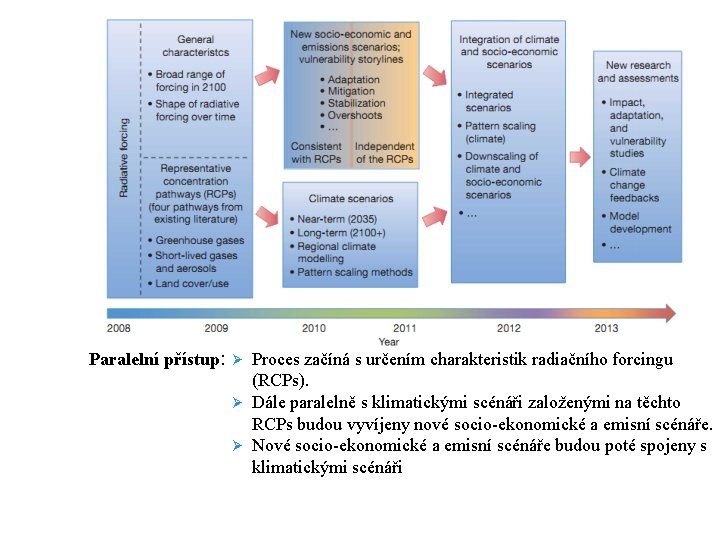
Paralelní přístup: Ø Proces začíná s určením charakteristik radiačního forcingu (RCPs). Ø Dále paralelně s klimatickými scénáři založenými na těchto RCPs budou vyvíjeny nové socio-ekonomické a emisní scénáře. Ø Nové socio-ekonomické a emisní scénáře budou poté spojeny s klimatickými scénáři

Nová generace scénářů Ø Tento paralelní přístup by měl zmenšit časovou prodlevu mezi vytvořením emisních scénářů, jejich využitím v klimatických modelech a aplikací klimatických scénářů do dopadových studií Ø RCPs mohou být dosaženy různými možnostmi socio-ekonomického vývoje. Ø Paralelní přístup pak umožňuje vyšetření otázky – jak by se mohl „vyvíjet svět“, aby bylo dosaženo konkrétní dráhy radiačního forcingu Ø V těchto nových studiích by měla být věnována větší pozornost na vyhodnocení adaptačních potřeb a zkoumání možností pro zmírnění klimatických změn

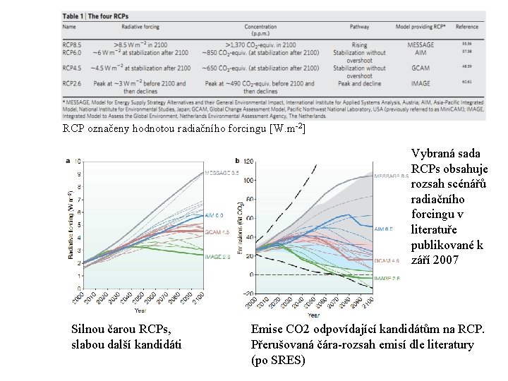
RCP označeny hodnotou radiačního forcingu [W. m-2] Vybraná sada RCPs obsahuje rozsah scénářů radiačního forcingu v literatuře publikované k září 2007 Silnou čarou RCPs, slabou další kandidáti Emise CO 2 odpovídající kandidátům na RCP. Přerušovaná čára-rozsah emisí dle literatury (po SRES)

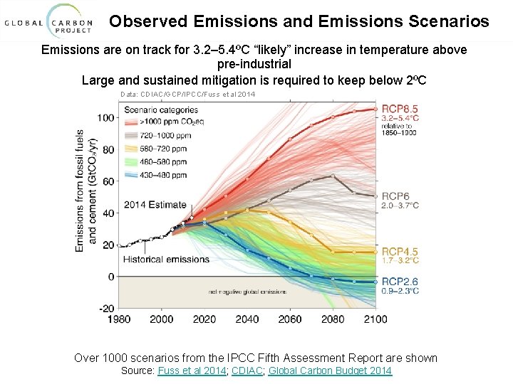
Observed Emissions and Emissions Scenarios Emissions are on track for 3. 2– 5. 4ºC “likely” increase in temperature above pre-industrial Large and sustained mitigation is required to keep below 2ºC Data: CDIAC/GCP/IPCC/Fuss et al 2014 Over 1000 scenarios from the IPCC Fifth Assessment Report are shown Source: Fuss et al 2014; CDIAC; Global Carbon Budget 2014

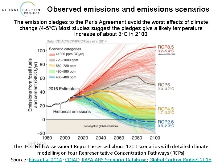
Observed emissions and emissions scenarios The emission pledges to the Paris Agreement avoid the worst effects of climate change (4 -5°C) Most studies suggest the pledges give a likely temperature increase of about 3°C in 2100 The IPCC Fifth Assessment Report assessed about 1200 scenarios with detailed climate modelling on four Representative Concentration Pathways (RCPs) Source: Fuss et al 2014; CDIAC; IIASA AR 5 Scenario Database; Global Carbon Budget 2016

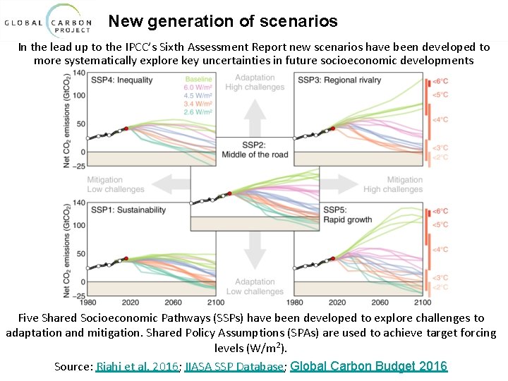
New generation of scenarios In the lead up to the IPCC’s Sixth Assessment Report new scenarios have been developed to more systematically explore key uncertainties in future socioeconomic developments Five Shared Socioeconomic Pathways (SSPs) have been developed to explore challenges to adaptation and mitigation. Shared Policy Assumptions (SPAs) are used to achieve target forcing levels (W/m 2). Source: Riahi et al. 2016; IIASA SSP Database; Global Carbon Budget 2016

Použitá literatura a odkazy Použitá literatura Ø Moss R. H. a kol. (2010): The next generation of scenarios for climate change and research, Nature, 463, 747 -755. Ø Moss R. H. a kol. (2007): Towards new scenarios for analysis of emissions, climate change, impacts and response strategies, IPCC expert meetin report – Technical summary, 463, 747 -755. Ø https: //www. gmes-atmosphere. eu/ Ø http: //www. ipcc. ch/report/ar 5/