UCST and LCST of polymers Binary Mixtures Consider

UCST and LCST of polymers

Binary Mixtures Consider a binary liquid mixture of n 1 + n 2 moles at fixed temperature and pressure. The necessary and sufficient condition for equilibrium is that the total Gibbs free energy of mixing, AG, for the mixture is a minimum with respect to all possible changes

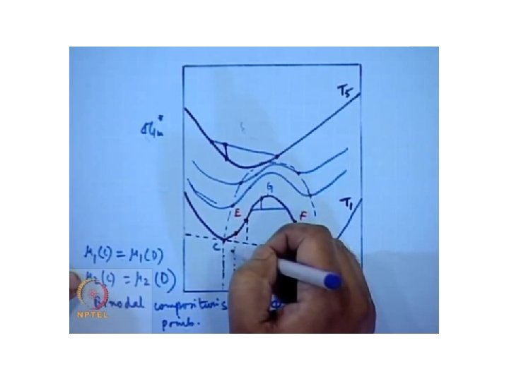
Figure 2 F-1. Gibbs Energy of Mixing as a Function of Volume Fraction. -—Hypothetical Predicted k. G-Curve in Two-Phase Region; Real LG-Curve

Tie line- straight line joining two points in that curve Let us take the curve T₅. and any point on the curve If this has to spontaneously phase separate to any composition. One has to be polymer rich and one has to be solvent rich.

This has to phase separate and comes to C &D Slight changes in the composition will be similar to T₅ the Gibb’s free energy will be positive so it would be stable for small changes in concentration. It is known as metastable region The system behaves as disscussed in T₅

Region between C to e and f to d any composition between e and f is completely unstable and will immediately phase separate into c and d. This is called inflection point.

Metastable region Metastable points

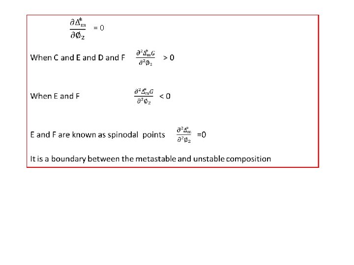
Phase separation C and d have a common tangent

Binodal points Ref. IIT Kharagpur nptel lectures by Prof. Dibankar Dhara

Metastable state Soluble at only these compositio ns Soluble at all compositions Completely in soluble

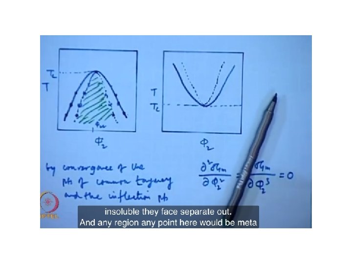
Locus points or coexistence points of binodal and spinnodal points and they merge at a point known as critical point. The critical point is the convergence of the points of common tangency and the inflection points.

Polymer Dissolution Phase Diagram • The extent of dissolution of a polymer in its solvent varies with the temperature as well as the extent of a good solvent mixed with a poor solvent • As the temperature of the polymer solvent mixture is raised , it turns transparent beyond a particular temperature and goes to a cloudy appearance (as observed in phenol water system) on ; lowering the temperature i. e the solution separates into two phases polymer and solvent. • The temperature at which both the phases coexist is called cloud point for that polymer solvent system at that particular concentration. (c)

• From the cloud point of a series of polymer solution of varying concentration from low to high will produce coexistence curve based on the phase diagram of the polymer solvent system. • Different polymer solvent system show different types of phase diagram.

UCST (polystyrene & cyclohexane) • Shows parabolic type of phase diagram. • The highest point in this coexistence curve on the temperature scale is referred to as the Tc or upper critical solution temperature (UCST). • And the corresponding concentration is called critical concentration for that system • Polymer solution is monophasic transparent at temperatures above the coexistence curve and become cloudy below the curve. • The coexistence curve is prepared by joining the Binodal points with minimum free energy of mixing

LCST (poly N-isopropyl acrylamide & water system) • It shows inverted parabola. Cloudy • The Tc is the lowest point biphasic on the coexistence curve and Coexistence thus the Tc for this polymer solvent system as Lower critical Monophasic solution temperature • The polymer soluble in water because of H-bonding show LCST type of phase diagram as the H-bonding undergoes disruption at elevated temperature • Polymer solution is biphasic transparent below the coexistence curve and becomes biphasic cloudy heated above the coexistence curve.

UCST • The system is monophasic transparent solution outside bur biphasic within the coexistence curve loop. • Both LCST and UCST types of system overlap each other. LCST • Example of this system include aqueous solutions of polyethylene glycol, polyhydroxy methylmethacrylate