U S Traffic Sign Recognition Using Deep Learning

U. S. Traffic Sign Recognition Using Deep Learning Networks BY: PETER MOLLICA

Overview Introduction Traffic Sign Recognition Overview Related Work Background Sliding Window Detector Current State-of-the-Art Detection Performance Integral Images Integral Channel Features / Aggregate Channel Features Ada. Boost Deep Learning Experiments & Data Experimental Setup Preliminary Results Timeline for Future Work

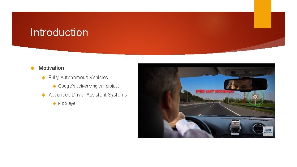
Introduction Motivation: Fully Autonomous Vehicles Google’s self-driving car project Advanced Driver Assistant Systems Mobileye

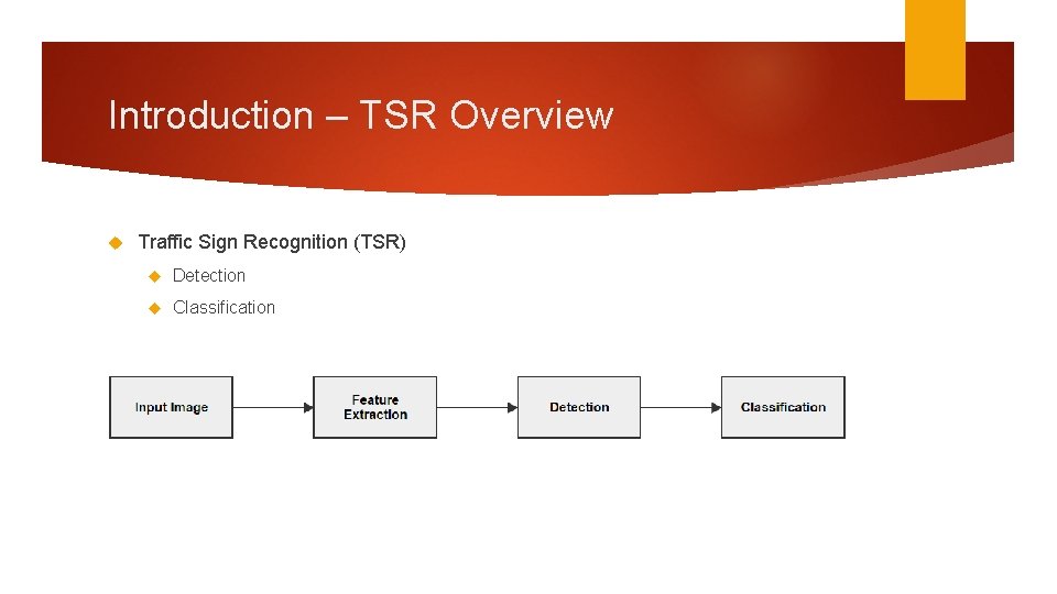
Introduction – TSR Overview Traffic Sign Recognition (TSR) Detection Classification

Introduction – TSR Overview U. S and European traffic sign datasets (publicly available): European (Vienna Convention): BTSD (Belgium Traffic Sign Data set) (2010) STS (Swedish Traffic Sign Data set) (2011) GTSRB (German Traffic Sign Recognition Benchmark) (2011) United States LISA (Laboratory for Intelligent and Safe Automobiles) (2012) Extension (2014)

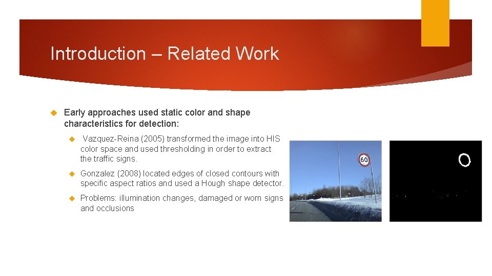
Introduction – Related Work Early approaches used static color and shape characteristics for detection: Vazquez-Reina (2005) transformed the image into HIS color space and used thresholding in order to extract the traffic signs. Gonzalez (2008) located edges of closed contours with specific aspect ratios and used a Hough shape detector. Problems: illumination changes, damaged or worn signs and occlusions

Introduction – Related Work Learning – based approaches became more popular: Creusen (2010) used HOG features with an SVM on a smaller self-generated dataset with good detection results. Overett (2011) used Various HOG features with a cascade classifier on a small New Zealand dataset with state-of-the-art detection performance. Problem: hard to evaluate performances of different methods when they are not evaluated on the same data set. This lead to the German Traffic Sign Recognition Benchmark competition (2013)

Introduction – Related Work German Traffic Sign Recognition Benchmark competition Detection: Team VISICS: Integral Channel Features. Team Litsi: HOG features and color histograms trained with a SVM. Team wgy@HIT 501: HOG features with LDA trained with an IK-SVM. Classification: Team IDSIA: Committee of CNNs Team sermanet: Multi-Scale CNNs Team CAOR: Random Forests

Introduction – Related Work Impressive Performances were achieved on the GTSRB datasets, however this does do not necessarily mean these methods will generalize well to U. S traffic signs. This led to the creation of the LISA dataset (Mogelmose 2013) largest publicly available U. S traffic sign dataset. Mogelmose demonstrated state-of-the-art performance on the LISA dataset using Aggregate Channel Features.

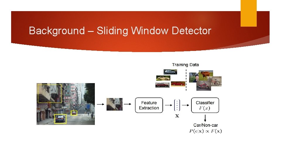
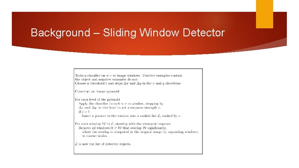
Background – Sliding Window Detector Most object recognition systems will typically implement a sliding window detector. The idea is to train a classifier on a certain size image patch. Slide a window across different scales of the input image. Extract features from the window. Feed the features to a classifier and determine if it is or isn’t the object we are looking for. Then apply non-maximum suppression.

Background – Sliding Window Detector

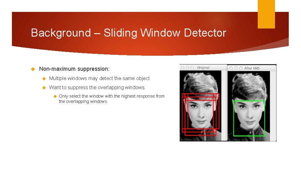
Background – Sliding Window Detector Non-maximum suppression: Multiple windows may detect the same object. Want to suppress the overlapping windows. Only select the window with the highest response from the overlapping windows.

Background – Sliding Window Detector

Background – Sliding Window Detector Evaluation: PASCAL meaurse

Background - Current State-of-the-Art Detection Performance Mogelmose (2015) has shown that Integral Channel Features (ICF) and Aggregate Channel features have achieved state-of-the-art detection performance for U. S traffic Signs. This method will be used as our baseline comparison.

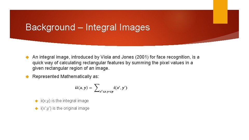
Background – Integral Images An integral image, introduced by Viola and Jones (2001) for face recognition, is a quick way of calculating rectangular features by summing the pixel values in a given rectangular region of an image. Represented Mathematically as: ii(x, y) is the integral image i(x’, y’) is the original image

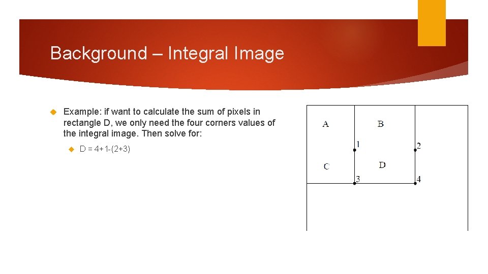
Background – Integral Image Example: if want to calculate the sum of pixels in rectangle D, we only need the four corners values of the integral image. Then solve for: D = 4+1 -(2+3)

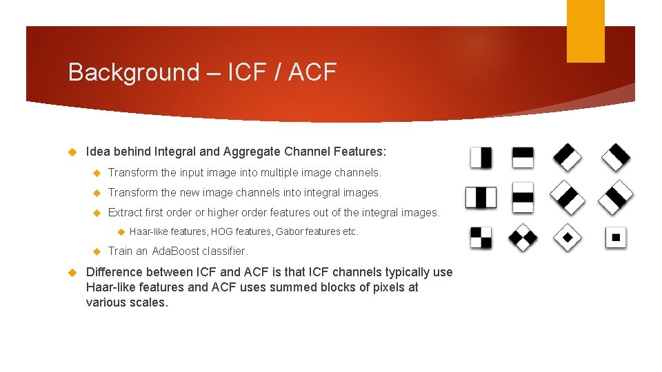
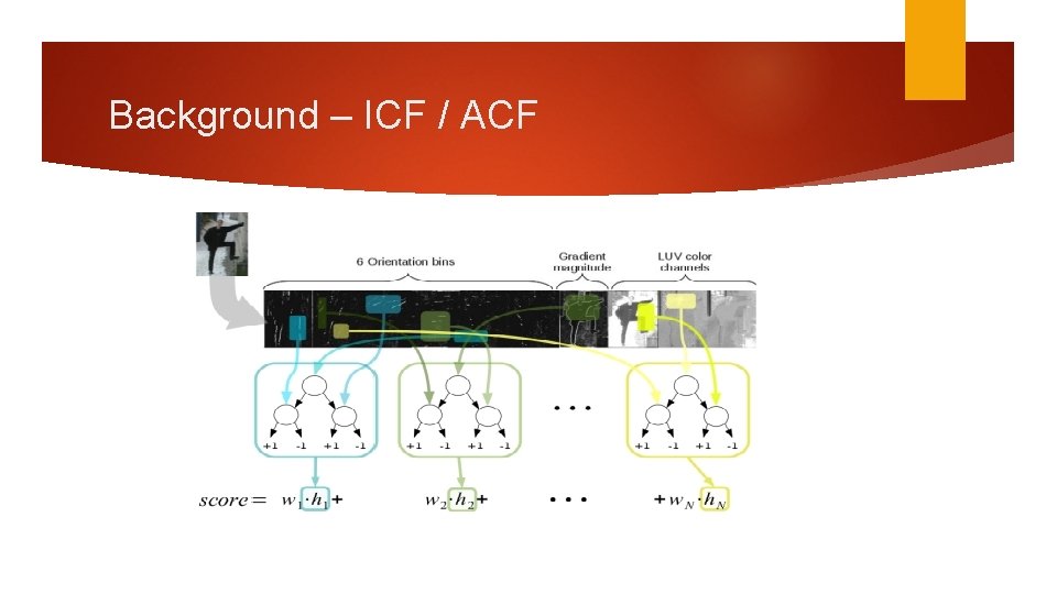
Background – ICF / ACF Idea behind Integral and Aggregate Channel Features: Transform the input image into multiple image channels. Transform the new image channels into integral images. Extract first order or higher order features out of the integral images. Haar-like features, HOG features, Gabor features etc. Train an Ada. Boost classifier. Difference between ICF and ACF is that ICF channels typically use Haar-like features and ACF uses summed blocks of pixels at various scales.

Background – ICF / ACF

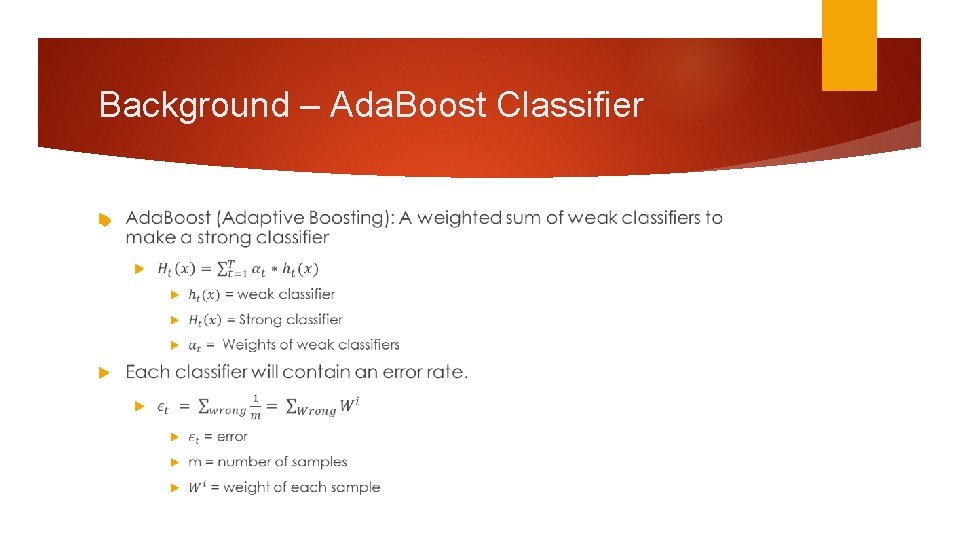
Background – Ada. Boost Classifier

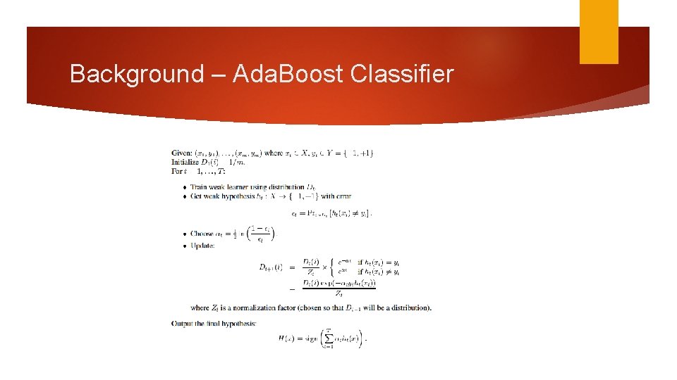
Background – Ada. Boost Classifier

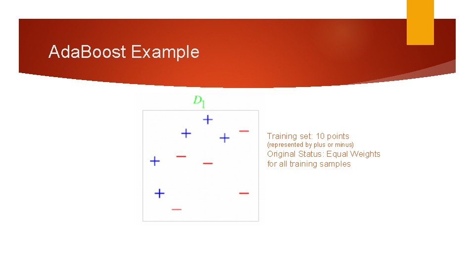
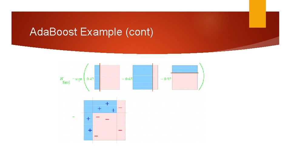
Ada. Boost Example Training set: 10 points (represented by plus or minus) Original Status: Equal Weights for all training samples

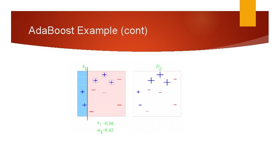
Ada. Boost Example (cont)

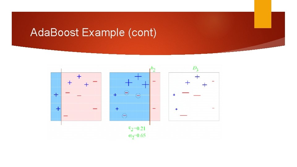
Ada. Boost Example (cont)

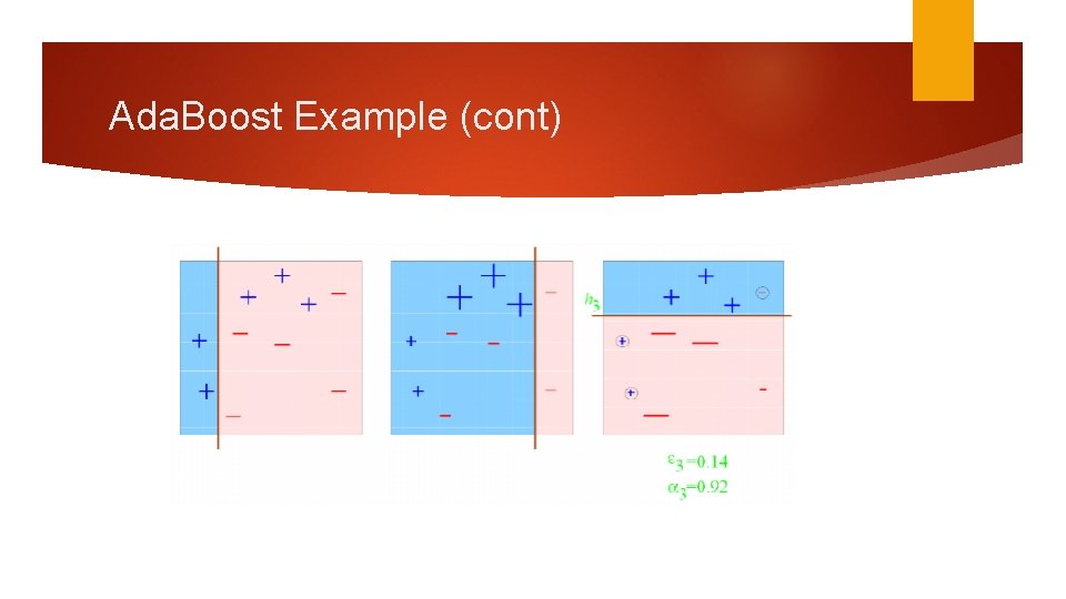
Ada. Boost Example (cont)

Ada. Boost Example (cont)

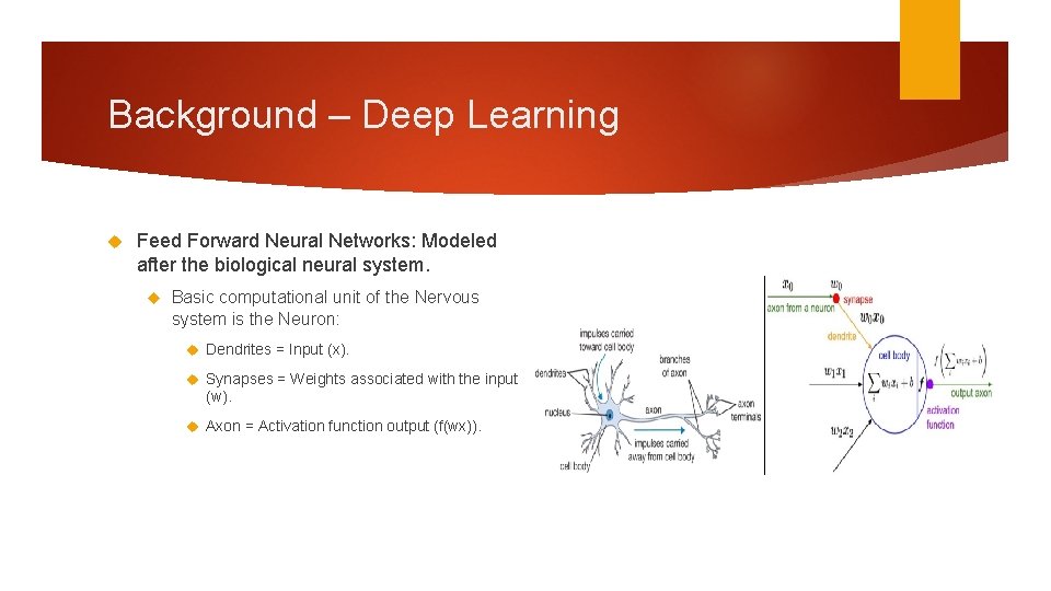
Background – Deep Learning Feed Forward Neural Networks: Modeled after the biological neural system. Basic computational unit of the Nervous system is the Neuron: Dendrites = Input (x). Synapses = Weights associated with the input (w). Axon = Activation function output (f(wx)).

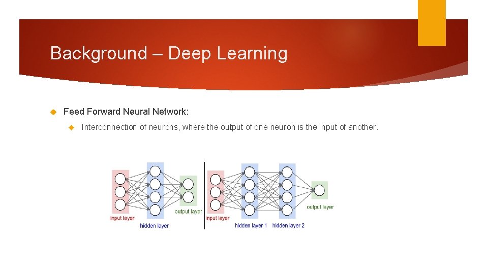
Background – Deep Learning Feed Forward Neural Network: Interconnection of neurons, where the output of one neuron is the input of another.

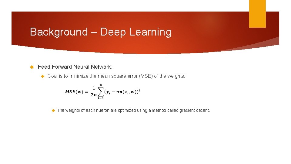
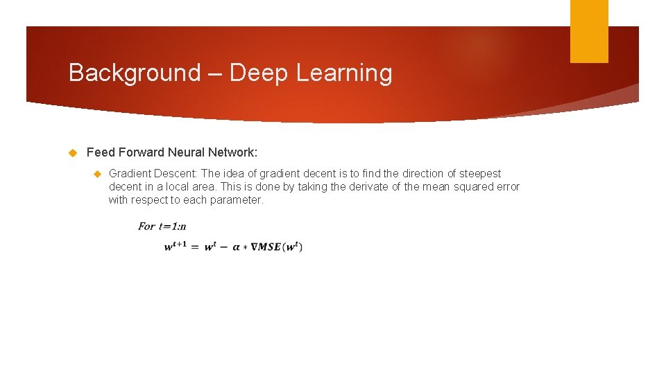
Background – Deep Learning Feed Forward Neural Network: Goal is to minimize the mean square error (MSE) of the weights: The weights of each nueron are optimized using a method called gradient decent.

Background – Deep Learning Feed Forward Neural Network: Gradient Descent: The idea of gradient decent is to find the direction of steepest decent in a local area. This is done by taking the derivate of the mean squared error with respect to each parameter.

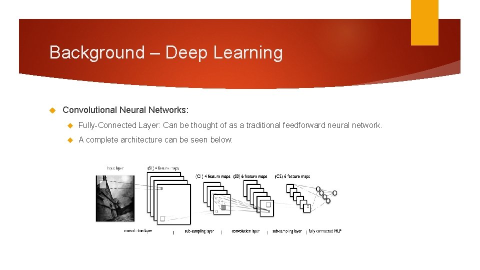
Background – Deep Learning Convolutional Neural Network (CNN): very similar to feedforward neural networks but are specialized for processing data with a grid-like topology, such as images. A basic CNN is composed of 3 main layers: Convolutional Layer Pooling Layer Fully-Connected Layer

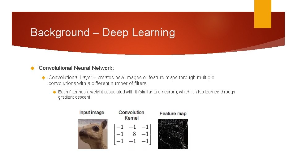
Background – Deep Learning Convolutional Neural Network: Convolutional Layer – creates new images or feature maps through multiple convolutions with a different number of filters. Each filter has a weight associated with it (similar to a neuron), which is also learned through gradient descent.

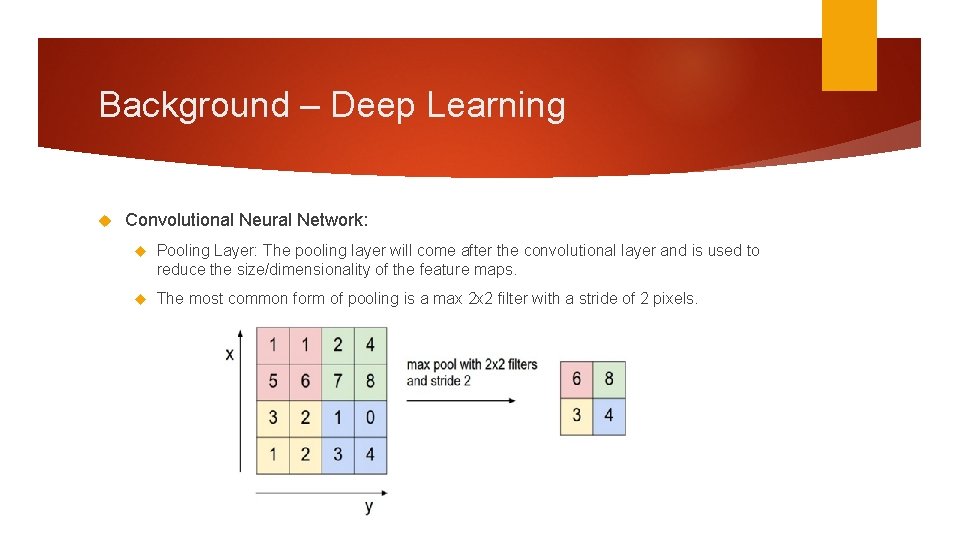
Background – Deep Learning Convolutional Neural Network: Pooling Layer: The pooling layer will come after the convolutional layer and is used to reduce the size/dimensionality of the feature maps. The most common form of pooling is a max 2 x 2 filter with a stride of 2 pixels.

Background – Deep Learning Convolutional Neural Networks: Fully-Connected Layer: Can be thought of as a traditional feedforward neural network. A complete architecture can be seen below:

Experiments & Data Proposal: The aim of this work is to do a comparative study of the current state-of -the-art methods for traffic sign detection and classification and compare them to different deep learning architectures. Ideally, design a single classifier that will be able to perform both the detection and classification of U. S traffic signs. The work proposed by Mogelmose (2015) for detection will be replicated and used as the baseline measurement

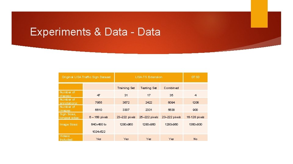
Experiments & Data - Data: The LISA dataset The original and extended dataset The German Traffic Sign Detection (GTSD) dataset

Experiments & Data - Data Original LISA Traffic Sign Dataset Number of classes: Number of annotations: Number of images: Sign Sizes, longest edge: Image Sizes: LISA-TS Extension GTSD Training Set Testing Set Combined 47 31 17 35 4 7855 3672 2422 6094 1206 6610 3307 2331 5638 900 6 – 168 pixels 23– 222 pixels 25– 222 pixels 23– 222 pixels 16 -128 pixels 640 x 480 to 1280 x 960 1360 x 800 Yes Yes No 1024 x 522 Videos Included: Yes

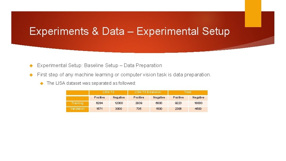
Experiments & Data – Experimental Setup: Baseline Setup – Data Preparation First step of any machine learning or computer vision task is data preparation. The LISA dataset was separated as followed: LISA-TS Extension Total Positive Negative Training 6284 12000 2939 6000 9223 18000 Validation 1571 3000 735 1500 2306 4500

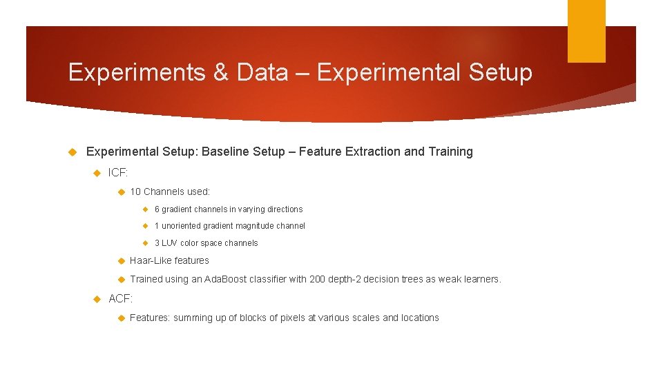
Experiments & Data – Experimental Setup: Baseline Setup – Feature Extraction and Training ICF: 10 Channels used: 6 gradient channels in varying directions 1 unoriented gradient magnitude channel 3 LUV color space channels Haar-Like features Trained using an Ada. Boost classifier with 200 depth-2 decision trees as weak learners. ACF: Features: summing up of blocks of pixels at various scales and locations

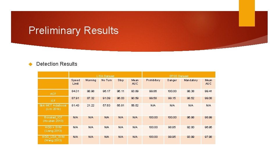
Preliminary Results Detection Results Speed Limit Warning 84. 31 98. 98 87. 91 8 bit-MCT Ada. Boost (Lim 2014) LISA Dataset No Turn GTSD Dataset Danger Mandatory Stop Mean AUC Prohibitory 96. 17 96. 11 93. 89 99. 86 100. 00 98. 38 99. 41 87. 32 91. 09 96. 03 90. 59 99. 58 99. 15 98. 52 99. 08 81. 43 21. 22 57. 63 65. 81 56. 52 N/A N/A Boosted_ICF (Houben 2013) N/A N/A N/A 100. 00 96. 98 98. 99 HOG + SVM (Liang 2013) N/A N/A N/A 100. 00 98. 85 92. 00 96. 95 HOG_LDA_SVM (Wang 2013) N/A N/A N/A 100. 00 99. 95 93. 99 97. 98 ACF ICF Mean AUC

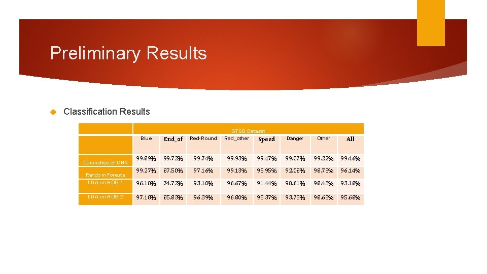
Preliminary Results Classification Results GTSD Dataset Red_other Speed Blue End_of Red-Round 99. 89% 99. 72% 99. 74% 99. 93% 99. 27% 87. 50% 97. 16% LDA on HOG 1 96. 10% 74. 72% LDA on HOG 2 97. 18% 85. 83% Committee of CNN Random Forests Danger Other All 99. 47% 99. 07% 99. 22% 99. 46% 99. 13% 95. 95% 92. 08% 98. 73% 96. 14% 93. 10% 96. 67% 91. 44% 90. 61% 98. 43% 93. 18% 96. 39% 96. 80% 95. 37% 93. 73% 98. 63% 95. 68%

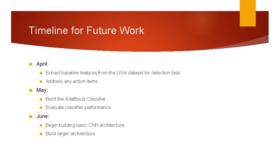
Timeline for Future Work April: Extract baseline features from the LISA dataset for detection task Address any action items May: Build the Ada. Boost Classifier. Evaluate classifier performance June: Begin building basic CNN architecture Build larger architecture

Timeline for Future Work July: Evaluate performance Experiment with different variations of CNNs August: Evaluate the Performance of new CNNs designs September-December Address any issues that may arise Finish a complete and final draft of thesis Successfully defend thesis

Questions?

References 1. Bishop, C. (2007). "Pattern Recognition and Machine Learning" (2 nd ed). New York, USA: Springer. 7. 2. Dalal, N. and Triggs, B. (2005) "Histograms of oriented gradients for human detection, " Computer Vision and Pattern Recognition, 2005. CVPR 2005. IEEE Computer Society Conference on, San Diego, CA, USA, 2005, pp. 886 -893 vol. 1. doi: 10. 1109/CVPR. 2005. 177 Freund, Y. and Schapire, R. E. (1996), ``Experiments with an new boosting algorithm, Machine Learning: Proceedings of the Thirteenth International Conference, Morgan Kauffman, San. Francisco, pp. 148156 (1996). Introduced Ada. Boost 8. Friedman, J. , Hastie, T. , and Tibshirani, R. (2000), “Additive Logistic. Regression: A Statistical View of Boosting, ” Annals of Statistics, vol. 38, no. 2, pp. 337 -374, 2000. 9. Forsyth, D. and Ponce, J. (2012). Computer Vision a Modern Approach (2 nd ed. , p. 549). New York, USA: Pearson 10. Houben, S. , Stallkamp, J. , Salmen, J. , Schlipsing, M. , and Igel, C. (2013), "Detection of traffic signs in real-world images: The German traffic sign detection benchmark, " Neural Networks (IJCNN), The 2013 International Joint Conference on, Dallas, TX, 2013, pp. 1 -8. doi: 10. 1109/IJCNN. 2013. 6706807 11. Krizhevsky, A. , Sutskever, I. , and Hinton, G. (2012), Imagenet classification with deep convolutional neural networks. In NIPS, 2012. 1, 2, 3, 4 3. Dollár, P. , “Piotr’s Computer Vision Matlab Toolbox (PMT). ” [Online]. Available: http: //vision. ucsd. edu/ignorespacespdollar/toolbox/doc/index. html 4. Dollar, P. , Appel, R. , Belongie, S. , and Perona, P. (2014), "Fast Feature Pyramids for Object Detection, " in IEEE Transactions on Pattern Analysis and Machine Intelligence, vol. 36, no. 8, pp. 15321545, Aug. 2014. doi: 10. 1109/TPAMI. 2014. 2300479 5. Dollár, P. , Tu, Z. , Perona, P. , and Belongie S. (2009), “Integral channel features, ” in Proc. BMVC, vol. 2, no. 3, p. 5, 200 6. Everingham, M. , Gool, L. , Williams, C. , Winn, J. , and Zisserman, A. (2010). The Pascal Visual Object Classes (VOC) Challenge. Int. J. 12. Comput. Vision 88, 2 (June 2010), 303 -338. DOI=http: //dx. doi. org/10. 1007/s 11263 -009 -0275 -4 13. Li, F. , Karpathy, A. , and Johnson, J. (2015), "CS 231 n: Convolutional Neural Networks for Visual Recognition, " www. http: //cs 231 n. stanford. edu/

References 14. Lim, K. , Lee, T. , Shin, C. , Chung, S. , Choi, Y. , and Byun, H. , (2014). Realtime illumination-invariant speed-limit sign recognition based on a modified census transform and support vector machines. In Proceedings of the 8 th International Conference on Ubiquitous Information Management and Communication (ICUIMC '14). ACM, New York, NY, USA, , Article 92 , 5 pages. DOI=http: //dx. doi. org/10. 1145/2557977. 2558090 15. Liu, W. , Wu, Y. , Lv, J. , Yuan, H. , and Zhao, H. (2012) "U. S. speed limit sign detection and recognition from image sequences, " Control Automation Robotics & Vision (ICARCV), 2012 12 th International Conference on, Guangzhou, 2012, pp. 1437 -1442. doi: 10. 1109/ICARCV. 2012. 6485388 16. Loy, G. and Barnes, N. (2004), “Fast shape-based road sign detection for a driver assistance system, ” in Proc. IEEE/RSJ Int. Conf. IROS, 2004, vol. 1, pp. 70– 75 17. 18. 19. 20. Staudenmaier, A. , Klauck, U. , Kreßel, U. , Lindner, F. , and Wöhler, C. (2012) “Confidence measurements for adaptive Bayes decision classifier cascades and their application to US speed limit detection, ” in Proc. Pattern Recognit. , ser. Lecture Notes in Computer Science, vol. 7476, pp. 478– 487, 2012. 21. Vázquez-Reina, A. , Lafuente-Arroyo, S. , Siegmann, P. , Maldonado. Bascón, S. , and Acevedo-Rodríguez, F. (2005), “Traffic sign shape classification based on correlation techniques, ” in Proc. 5 th WSEAS Int. Conf. Signal Process. , Comput. Geometry Artif. Vis. , 2005, pp. 149– 154. 22. Mogelmose, A. , Liu, D. , and Trivedi, M. M. (2015), "Detection of U. S. Traffic Signs, " in IEEE Transactions on Intelligent Transportation Systems, vol. 16, no. 6, pp. 3116 -3125, Dec. 2015. doi: 10. 1109/TITS. 2015. 2433019 Viola, P. and Jones, M. (2001), "Rapid object detection using a boosted cascade of simple features, " Computer Vision and Pattern Recognition, 2001. CVPR 2001. Proceedings of the 2001 IEEE Computer Society Conference on, 2001, pp. I-511 -I-518 vol. 1. doi: 10. 1109/CVPR. 2001. 990517 23. Mogelmose, A. , Liu, D. , and Trivedi, M. M. (2014), "Traffic sign detection for U. S. roads: Remaining challenges and a case for tracking, " Intelligent Transportation Systems (ITSC), 2014 IEEE 17 th International Conference on, Qingdao, 2014, pp. 1394 -1399. doi: 10. 1109/ITSC. 2014. 6957882 Wang, G. , Ren, G. , Wu, Z. , Zhao, Y. , and Jiang, L. (2013), “A robust, coarse-to- fine traffic sign detection method, ” in Proc. IEEE IJCNN, Aug. 2013, pp. 1– 5. 24. United Nations (1978), "Vienna Convention on road signs and signals, “ 25. Zimmerman, A (2012), "Category-level Localization", Visual Geometry Group University of Oxford, http: //www. robots. ox. ac. uk/~vgg Mogelmose, A. , Trivedi, M. M. , and Moeslund, T. B. (2012), "Vision-Based Traffic Sign Detection and Analysis for Intelligent Driver Assistance Systems: Perspectives and Survey, " in IEEE Transactions on Intelligent Transportation Systems, vol. 13, no. 4, pp. 1484 -1497, Dec. 2012. doi: 10. 1109/TITS. 2012. 220942