U S Bureau of Labor Statistics Do Poor
U. S. Bureau of Labor Statistics Do Poor Pay More, Store by Store? Greg Kurtzon Robert Mc. Clelland Preliminary and Incomplete We thank Aylin Kumcu for her assistance with this research. All errors are our own. All views expressed in this paper are those of the authors and do not necessarily reflect the views or policies of the U. S. Bureau of Labor Statistics.
Do people with different incomes face different prices? • The poor pay more because they – are less mobile – shop at small, independent stores (not chains, not club stores) – shop in areas with higher insurance and security costs • The poor pay less because they – – have a lower opportunity cost of time buy lower quality products shop in areas with lower wages shop in outlets with fewer amenities 2

Real income distributions Some analyses conclude that the distribution of income has been widening The ‘real’ income distribution may not be as wide, or may be wider, than the ‘nominal’ distribution suggests 3
Previous literature • Caplovitz (1963) “The Poor Pay More” • BLS (1965) – independent stores, patronized by low income families, charge more • Summary in Sexton (1971) – no difference, or poor pay more • Summary in in Kaufman, et. Al. , (1997) – no difference, or poor pay more • Hayes (2000) • Aguiar and Hurst (2005) 4
Previous literature Hayes (2000) uses BLS 1998 micro-data for six homogeneous goods, and finds that prices for a set of homogeneous items sold in ‘poor’ areas are up to 6% lower. ‘Poor’ is defined by characteristics at the zip code and county level Aguiar and Hurst (2005) use AC Nielsen ‘Homescan’ data for Denver 1993 -5. 85% of purchases come from four chains. They conclude that poor pay about 5% less 5
Data • We use the telephone point of purchase survey (TPOPS) to determine how much households with different incomes spend at specific outlets • That information, combined with price data is used to construct average prices levels for different incomes • We don’t have data on the purchasing patterns of different households within an outlet 6
TPOPS • Quarterly survey of around 15, 000 consumer units, contacted randomly by phone • Respondents are asked for recent (recall period varies by good) dollar expenditures on one of 16 POPS groups for each outlet shopped at – One POPS group asked for each PSU each quarter – Full rotation every 4 years – One consumer unit intended to stay in for 4 quarters 7
TPOPS In 2001 only, respondents were asked to place their consumer unit in one of three income groups: – 1 Lower less than $8, 000 for CUSIZE < 2; less than $18, 000 for CUSIZE = 3; less than $24, 000 for CUSIZE > 3 – 2 Middle $8, 000 -$30, 000 for CUSIZE < 2; $18, 000 -$57, 000 for CUSIZE = 2; $18, 000 -$64, 000 for CUSIZE = 3; $24, 000 -$66, 000 for CUSIZE > 3 – 3 Upper greater than $30, 000 for CUSIZE < 2; greater than $57, 000 for CUSIZE = 2; greater than $64, 000 for CUSIZE = 3; greater than $66, 000 for CUSIZE > 3 About 15% group 1, 50% group 2, 35% group 3 8
TPOPS • Only first time interviewees were asked the question, with around an 80% response rate • Therefore, an income group can be assigned to at least some respondents in quarters 2001 Q 1 – 2002 Q 3 • The quarter with the most respondents with an assigned income group is 2001 Q 4, about 55% • The attrition rate is around 17% per quarter, could be a bit high • Replacements are not asked income question • Outlet income group weights – For each outlet in the 2001 Q 1 – 2002 Q 3 TPOPS sample, total expenditures for each income group were calculated – Many outlets have only one or two consumer units shopping there 9
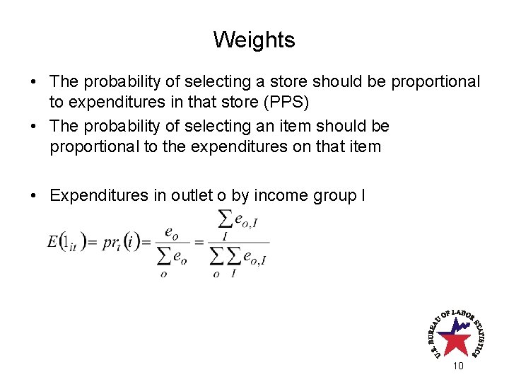
Weights • The probability of selecting a store should be proportional to expenditures in that store (PPS) • The probability of selecting an item should be proportional to the expenditures on that item • Expenditures in outlet o by income group I 10
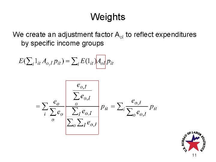
Weights We create an adjustment factor Ao. I to reflect expenditures by specific income groups 11
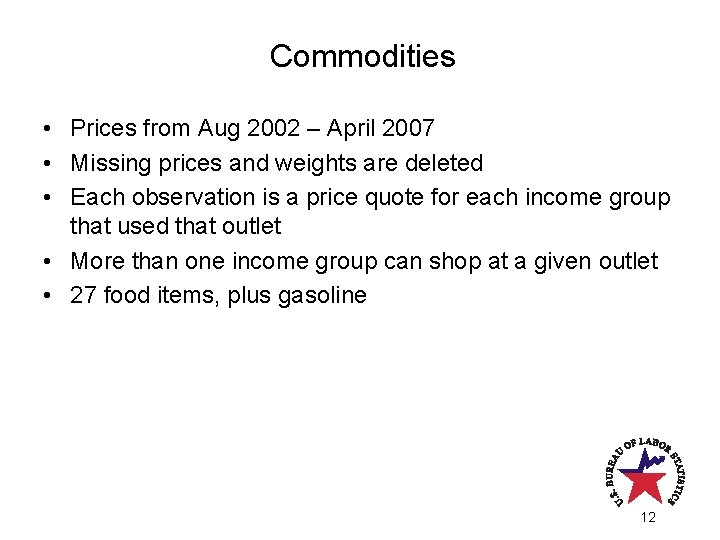
Commodities • Prices from Aug 2002 – April 2007 • Missing prices and weights are deleted • Each observation is a price quote for each income group that used that outlet • More than one income group can shop at a given outlet • 27 food items, plus gasoline 12
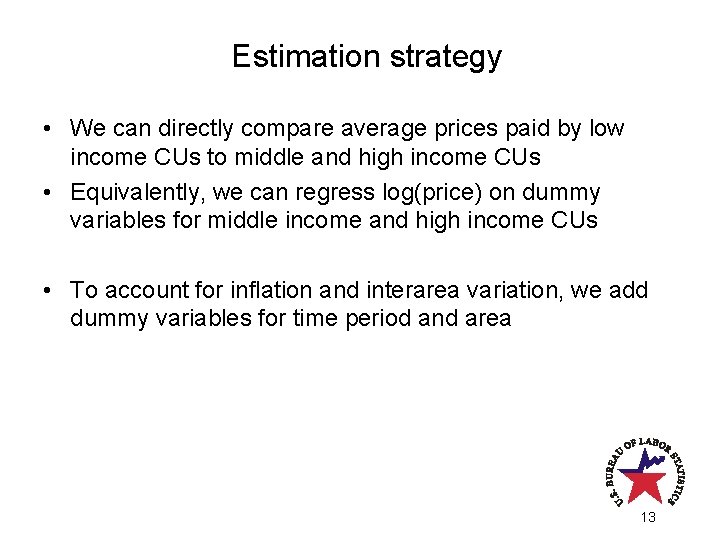
Estimation strategy • We can directly compare average prices paid by low income CUs to middle and high income CUs • Equivalently, we can regress log(price) on dummy variables for middle income and high income CUs • To account for inflation and interarea variation, we add dummy variables for time period and area 13
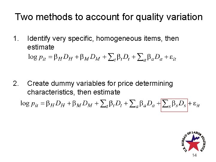
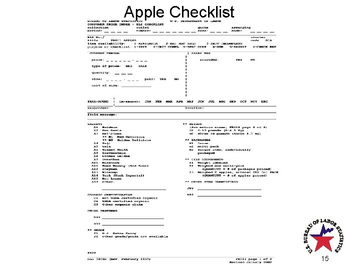
Two methods to account for quality variation 1. Identify very specific, homogeneous items, then estimate 2. Create dummy variables for price determining characteristics, then estimate 14
Apple Checklist 15

Examples of homogeneous items • National brand white bread, regular, not buttertop/salt free/dietetic/etc, not frozen, pre-pkged, 24 oz • National brand, chicken half breasts, skinless, fresh, no seasoning • National brand iceberg lettuce, single item package • National brand bacon, reg slice, not low salt, not smoked, not maple flavored or brown sugar cured • National brand bleached white all-purpose flour 5 lb 16
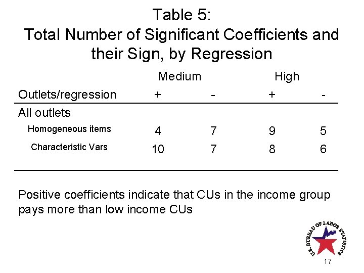
Table 5: Total Number of Significant Coefficients and their Sign, by Regression Medium + - High + - Homogeneous items 4 7 9 5 Characteristic Vars 10 7 8 6 Outlets/regression All outlets Positive coefficients indicate that CUs in the income group pays more than low income CUs 17
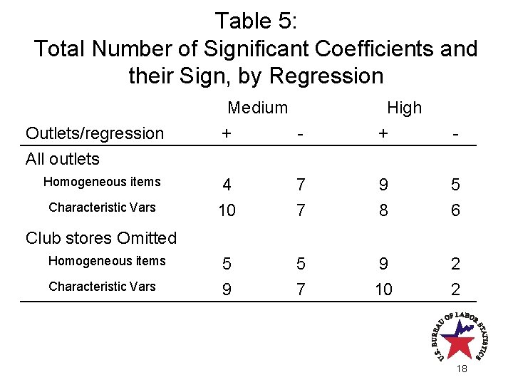
Table 5: Total Number of Significant Coefficients and their Sign, by Regression Medium + - High + - Homogeneous items 4 7 9 5 Characteristic Vars 10 7 8 6 5 9 5 7 9 10 2 2 Outlets/regression All outlets Club stores Omitted Homogeneous items Characteristic Vars 18
- Slides: 18