Types of risk Market risk Risk of losses
- Slides: 28

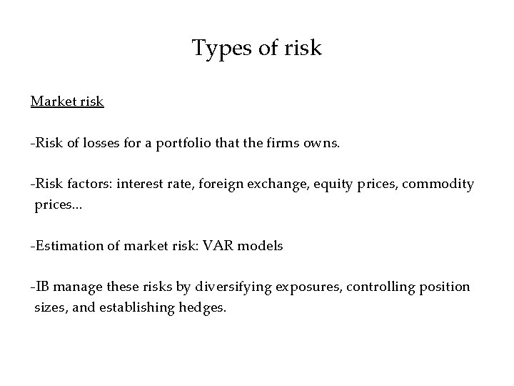
Types of risk Market risk -Risk of losses for a portfolio that the firms owns. -Risk factors: interest rate, foreign exchange, equity prices, commodity prices. . . -Estimation of market risk: VAR models -IB manage these risks by diversifying exposures, controlling position sizes, and establishing hedges.

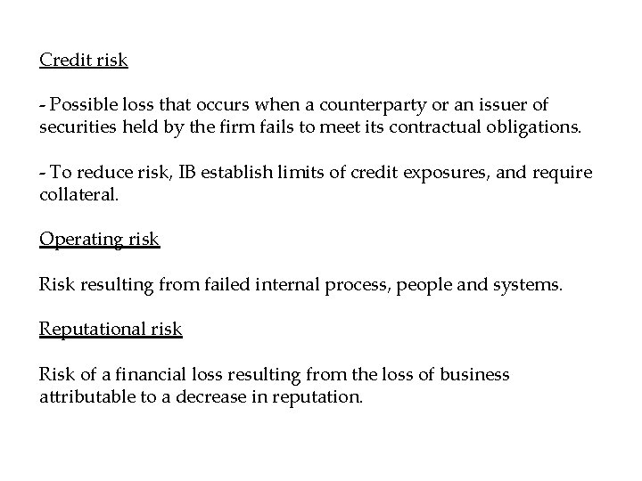
Credit risk - Possible loss that occurs when a counterparty or an issuer of securities held by the firm fails to meet its contractual obligations. - To reduce risk, IB establish limits of credit exposures, and require collateral. Operating risk Risk resulting from failed internal process, people and systems. Reputational risk Risk of a financial loss resulting from the loss of business attributable to a decrease in reputation.

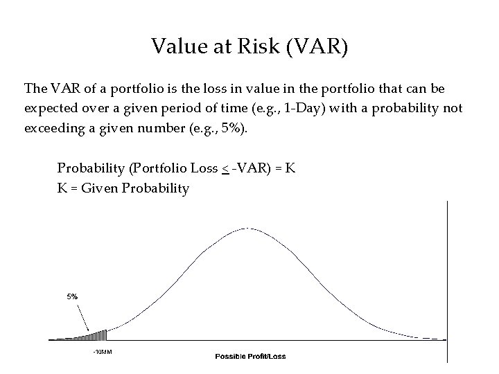
Value at Risk (VAR) The VAR of a portfolio is the loss in value in the portfolio that can be expected over a given period of time (e. g. , 1 -Day) with a probability not exceeding a given number (e. g. , 5%). Probability (Portfolio Loss < -VAR) = K K = Given Probability

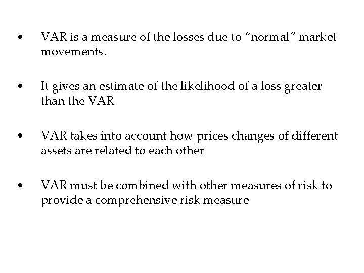
• VAR is a measure of the losses due to “normal” market movements. • It gives an estimate of the likelihood of a loss greater than the VAR • VAR takes into account how prices changes of different assets are related to each other • VAR must be combined with other measures of risk to provide a comprehensive risk measure

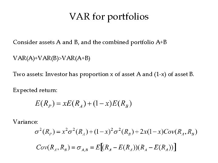
VAR for portfolios Consider assets A and B, and the combined portfolio A+B VAR(A)+VAR(B)>VAR(A+B) Two assets: Investor has proportion x of asset A and (1 -x) of asset B. Expected return: Variance:

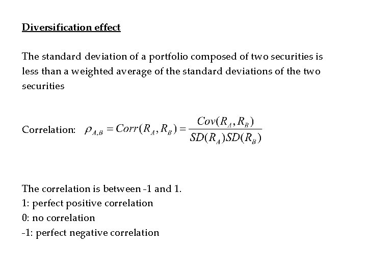
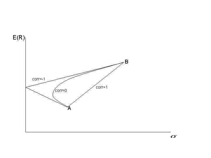
Diversification effect The standard deviation of a portfolio composed of two securities is less than a weighted average of the standard deviations of the two securities Correlation: The correlation is between -1 and 1. 1: perfect positive correlation 0: no correlation -1: perfect negative correlation

E(R) B corr=-1 corr=0 A

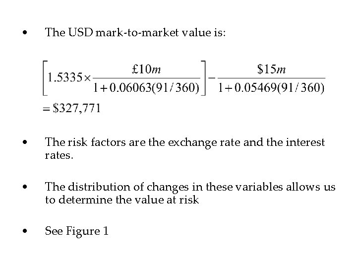
Example: Consider a forward contract: On delivery you will deliver $15 m and receive £ 10 m. At date t the contract has 91 days remaining until delivery. The 3 -month $ and £ interest rates are 5. 469% and 6. 063% respectively. The spot exchange rate is S=1. 5335$/£.

• The USD mark-to-market value is: • The risk factors are the exchange rate and the interest rates. • The distribution of changes in these variables allows us to determine the value at risk • See Figure 1

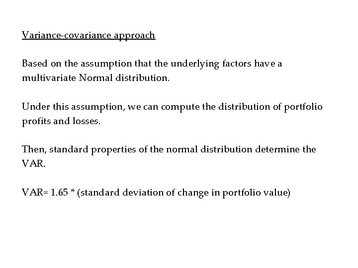
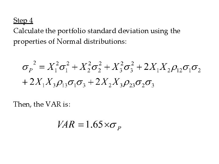
Variance-covariance approach Based on the assumption that the underlying factors have a multivariate Normal distribution. Under this assumption, we can compute the distribution of portfolio profits and losses. Then, standard properties of the normal distribution determine the VAR= 1. 65 * (standard deviation of change in portfolio value)

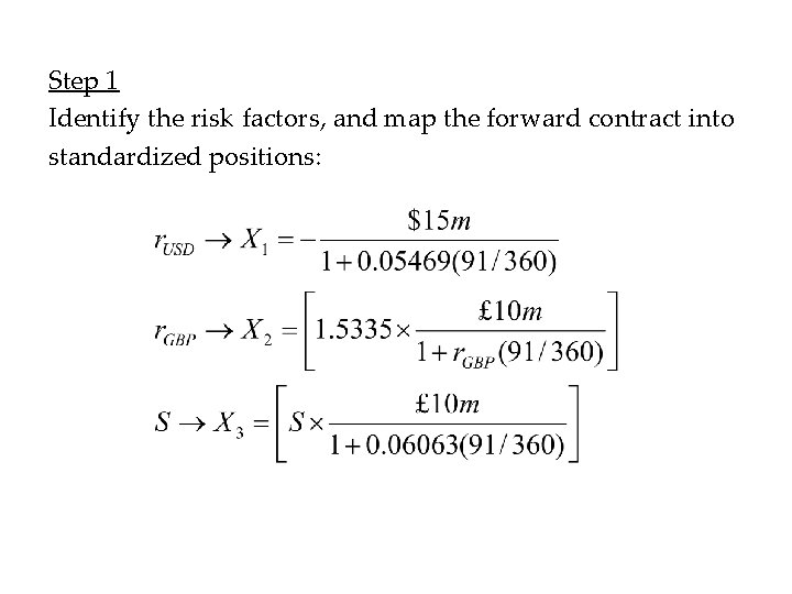
Step 1 Identify the risk factors, and map the forward contract into standardized positions:

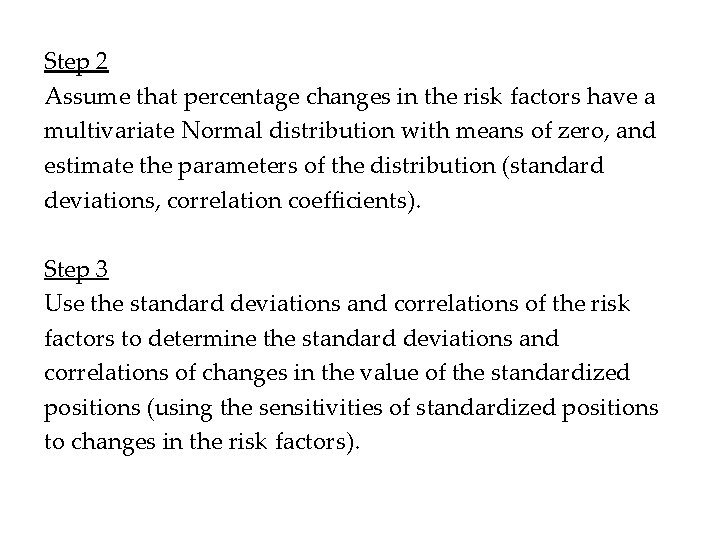
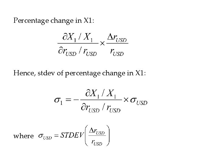
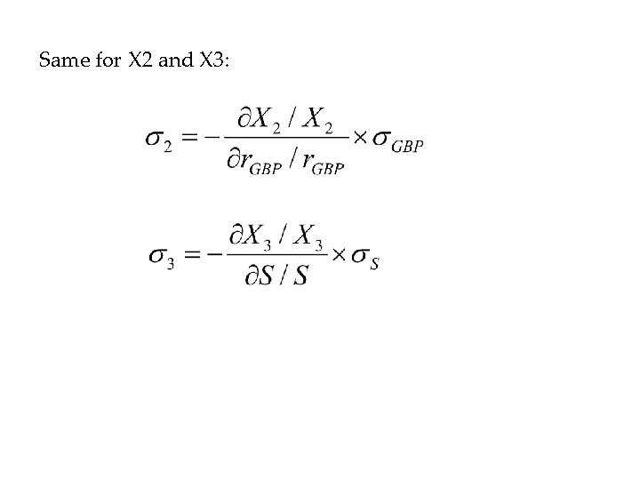
Step 2 Assume that percentage changes in the risk factors have a multivariate Normal distribution with means of zero, and estimate the parameters of the distribution (standard deviations, correlation coefficients). Step 3 Use the standard deviations and correlations of the risk factors to determine the standard deviations and correlations of changes in the value of the standardized positions (using the sensitivities of standardized positions to changes in the risk factors).

Percentage change in X 1: Hence, stdev of percentage change in X 1: where

Same for X 2 and X 3:

Step 4 Calculate the portfolio standard deviation using the properties of Normal distributions: Then, the VAR is:

Historical simulation Simple atheoretical approach, that requires relatively few assumptions. It consists of using historical changes in market rates and prices to construct a distribution of potential future profits and losses. The distribution of profits and losses takes the current portfolio, subjecting it to actual changes in risk factors experienced in the past N periods (trade-off regarding N). We calculate N historical percentage changes in risk factors, and see how these changes would affect the portfolio value today.

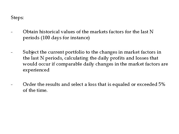
Steps: - Obtain historical values of the markets factors for the last N periods (100 days for instance) - Subject the current portfolio to the changes in market factors in the last N periods, calculating the daily profits and losses that would occur if comparable daily changes in the market factors are experienced - Order the results and select a loss that is equaled or exceeded 5% of the time.

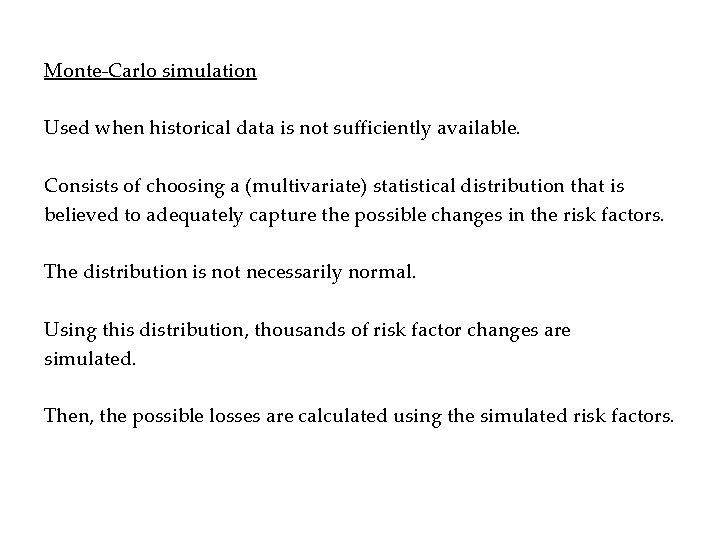
Monte-Carlo simulation Used when historical data is not sufficiently available. Consists of choosing a (multivariate) statistical distribution that is believed to adequately capture the possible changes in the risk factors. The distribution is not necessarily normal. Using this distribution, thousands of risk factor changes are simulated. Then, the possible losses are calculated using the simulated risk factors.

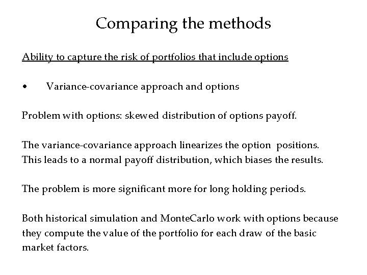
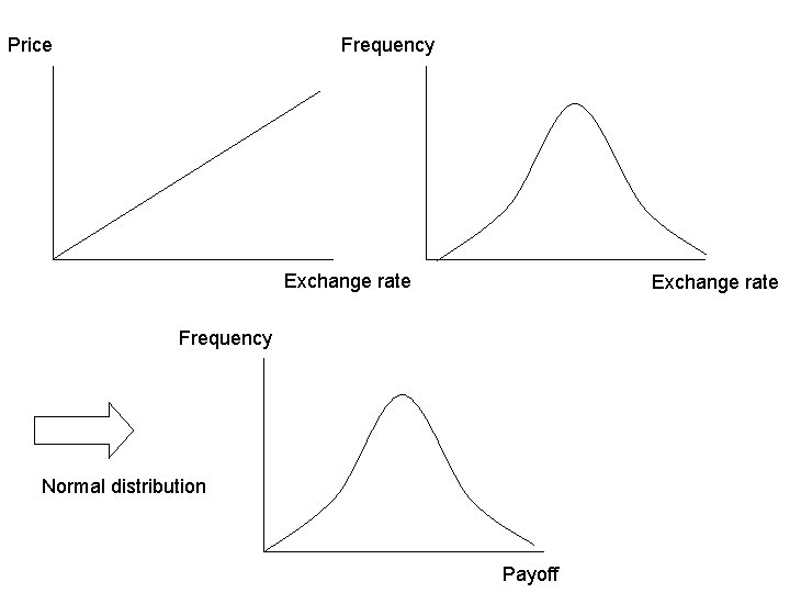
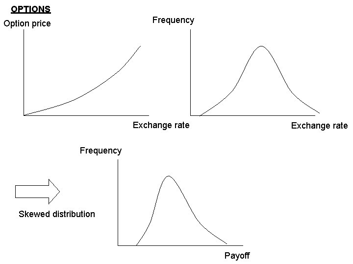
Comparing the methods Ability to capture the risk of portfolios that include options • Variance-covariance approach and options Problem with options: skewed distribution of options payoff. The variance-covariance approach linearizes the option positions. This leads to a normal payoff distribution, which biases the results. The problem is more significant more for long holding periods. Both historical simulation and Monte. Carlo work with options because they compute the value of the portfolio for each draw of the basic market factors.

Price Frequency Exchange rate Frequency Normal distribution Payoff

OPTIONS Frequency Option price Exchange rate Frequency Skewed distribution Payoff

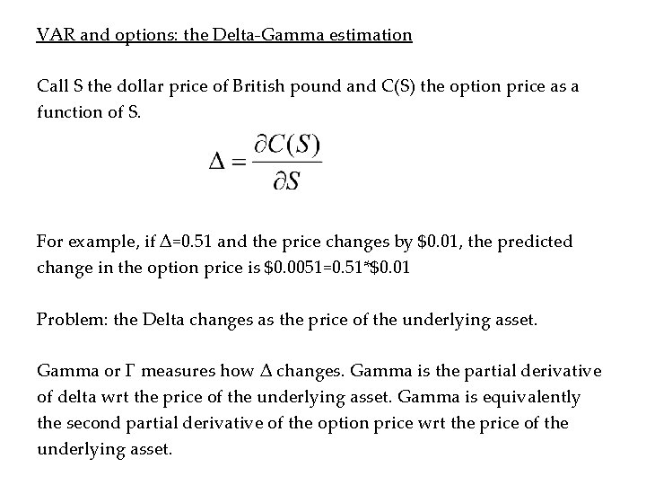
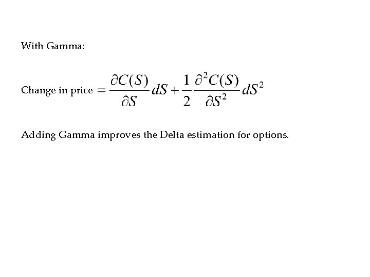
VAR and options: the Delta-Gamma estimation Call S the dollar price of British pound and C(S) the option price as a function of S. For example, if Δ=0. 51 and the price changes by $0. 01, the predicted change in the option price is $0. 0051=0. 51*$0. 01 Problem: the Delta changes as the price of the underlying asset. Gamma or Γ measures how Δ changes. Gamma is the partial derivative of delta wrt the price of the underlying asset. Gamma is equivalently the second partial derivative of the option price wrt the price of the underlying asset.

With Gamma: Change in price Adding Gamma improves the Delta estimation for options.

Generalities on the reliability of the results • For historical simulation, there is the risk that recent history is not typical (volatility). • Other methodologies also use historical data, but by assuming particular distributions, limit the possible shape that the estimated distribution can have. • Variance-covariance and Monte. Carlo approaches: the assumed distributions do not necessarily correspond to the true distributions (fat tails. . . ).

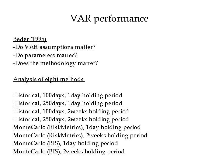
VAR performance Beder (1995) -Do VAR assumptions matter? -Do parameters matter? -Does the methodology matter? Analysis of eight methods: Historical, 100 days, 1 day holding period Historical, 250 days, 1 day holding period Historical, 100 days, 2 weeks holding period Historical, 250 days, 2 weeks holding period Monte. Carlo (Risk. Metrics), 1 day holding period Monte. Carlo (Risk. Metrics), 2 weeks holding period Monte. Carlo (BIS), 1 day holding period Monte. Carlo (BIS), 2 weeks holding period

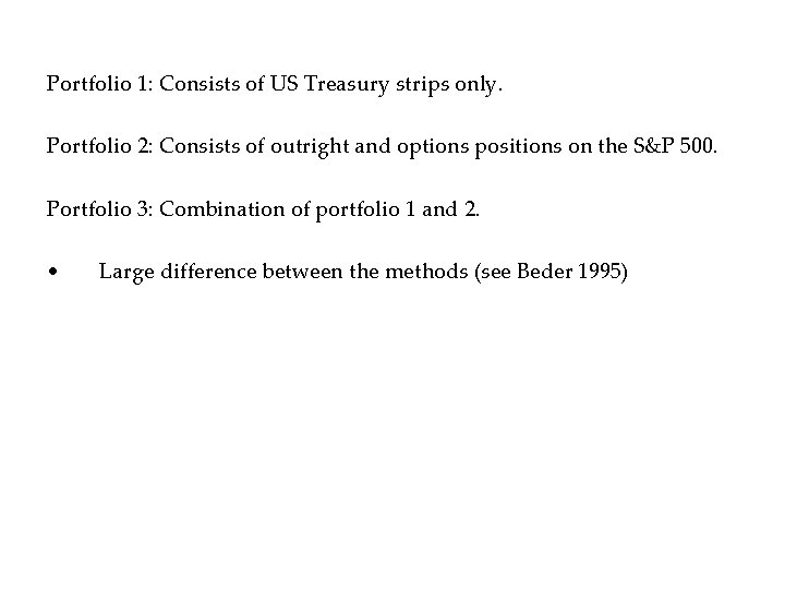
Portfolio 1: Consists of US Treasury strips only. Portfolio 2: Consists of outright and options positions on the S&P 500. Portfolio 3: Combination of portfolio 1 and 2. • Large difference between the methods (see Beder 1995)

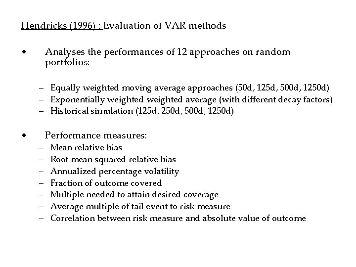
Hendricks (1996) : Evaluation of VAR methods • Analyses the performances of 12 approaches on random portfolios: – Equally weighted moving average approaches (50 d, 125 d, 500 d, 1250 d) – Exponentially weighted average (with different decay factors) – Historical simulation (125 d, 250 d, 500 d, 1250 d) • – – – – Performance measures: Mean relative bias Root mean squared relative bias Annualized percentage volatility Fraction of outcome covered Multiple needed to attain desired coverage Average multiple of tail event to risk measure Correlation between risk measure and absolute value of outcome

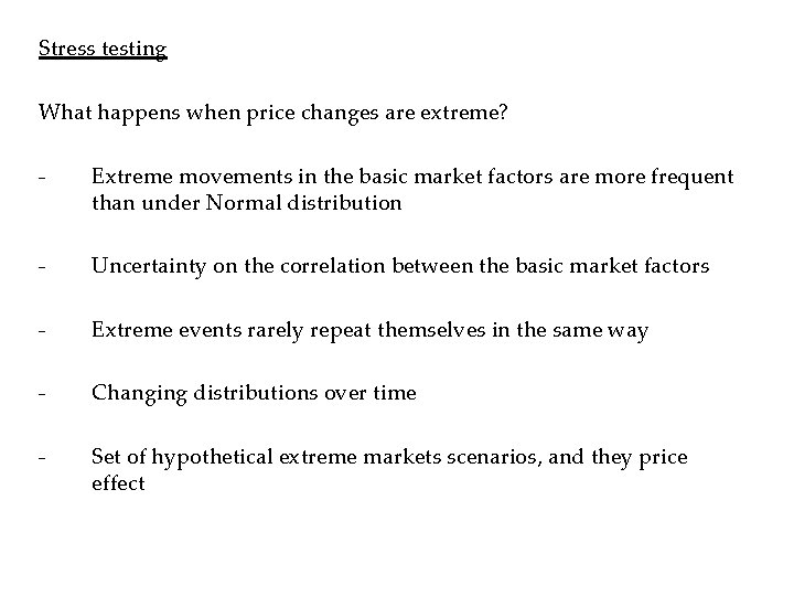
Stress testing What happens when price changes are extreme? - Extreme movements in the basic market factors are more frequent than under Normal distribution - Uncertainty on the correlation between the basic market factors - Extreme events rarely repeat themselves in the same way - Changing distributions over time - Set of hypothetical extreme markets scenarios, and they price effect