Types of analysis Simulation rationale u Each patients

Types of analysis

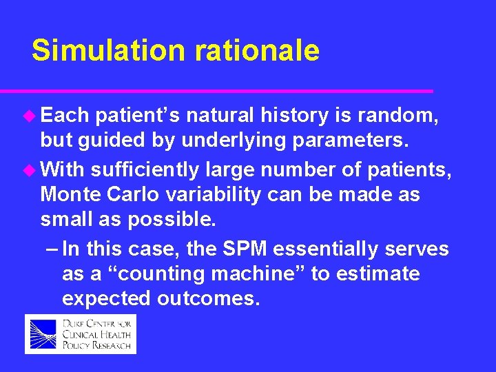
Simulation rationale u Each patient’s natural history is random, but guided by underlying parameters. u With sufficiently large number of patients, Monte Carlo variability can be made as small as possible. – In this case, the SPM essentially serves as a “counting machine” to estimate expected outcomes.

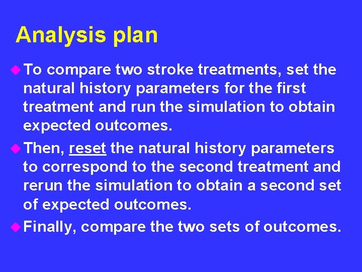
Analysis plan u To compare two stroke treatments, set the natural history parameters for the first treatment and run the simulation to obtain expected outcomes. u Then, reset the natural history parameters to correspond to the second treatment and rerun the simulation to obtain a second set of expected outcomes. u Finally, compare the two sets of outcomes.

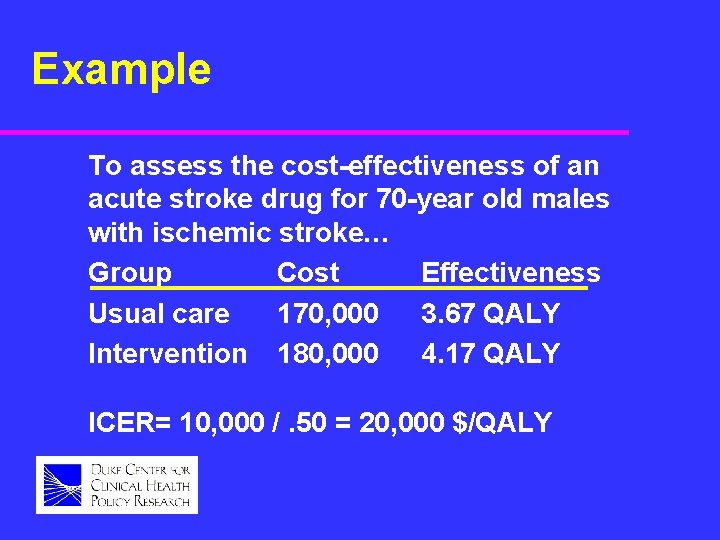
Example To assess the cost-effectiveness of an acute stroke drug for 70 -year old males with ischemic stroke… Group Cost Effectiveness Usual care 170, 000 3. 67 QALY Intervention 180, 000 4. 17 QALY ICER= 10, 000 /. 50 = 20, 000 $/QALY

Types of analysis u Base case u Sensitivity u Bootstrapping u Stochastic sensitivity u ……. .

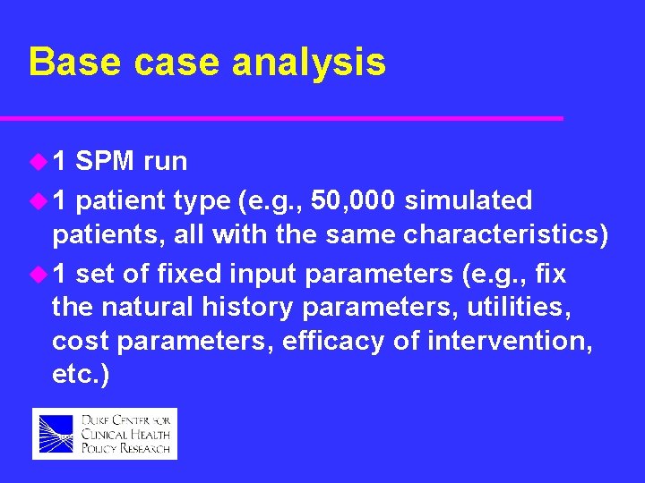
Base case analysis u 1 SPM run u 1 patient type (e. g. , 50, 000 simulated patients, all with the same characteristics) u 1 set of fixed input parameters (e. g. , fix the natural history parameters, utilities, cost parameters, efficacy of intervention, etc. )

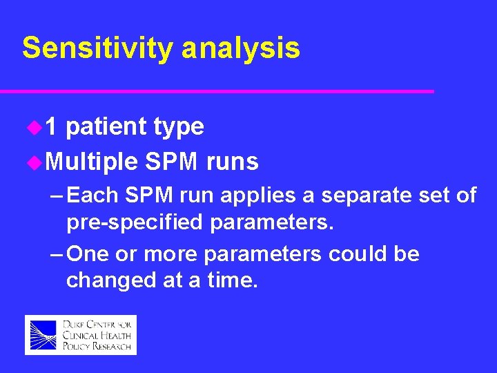
Sensitivity analysis u 1 patient type u. Multiple SPM runs – Each SPM run applies a separate set of pre-specified parameters. – One or more parameters could be changed at a time.

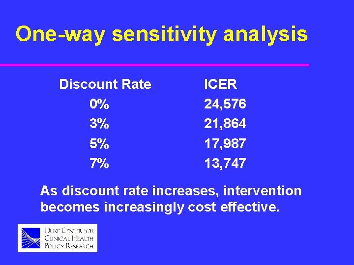
One-way sensitivity analysis Discount Rate 0% 3% 5% 7% ICER 24, 576 21, 864 17, 987 13, 747 As discount rate increases, intervention becomes increasingly cost effective.

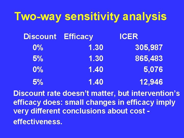
Two-way sensitivity analysis Discount Efficacy 0% 1. 30 5% 1. 30 0% 1. 40 ICER 305, 987 865, 483 5, 076 5% 1. 40 12, 946 Discount rate doesn’t matter, but intervention’s efficacy does: small changes in efficacy imply very different conclusions about cost effectiveness.

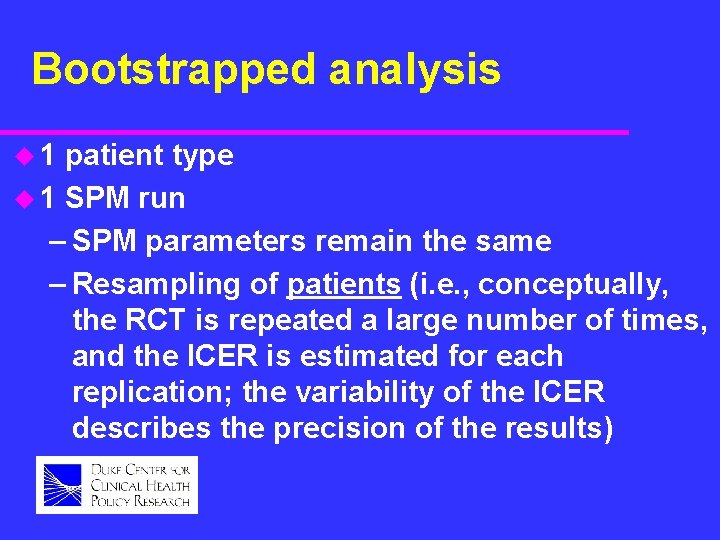
Bootstrapped analysis u 1 patient type u 1 SPM run – SPM parameters remain the same – Resampling of patients (i. e. , conceptually, the RCT is repeated a large number of times, and the ICER is estimated for each replication; the variability of the ICER describes the precision of the results)

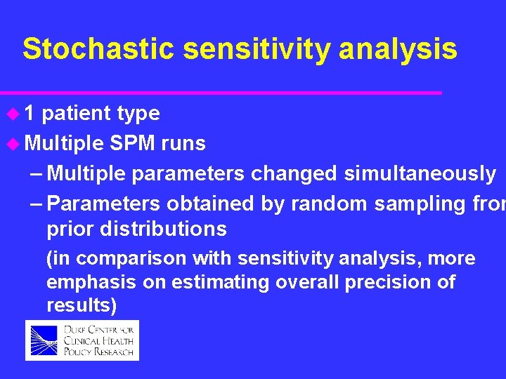
Stochastic sensitivity analysis u 1 patient type u Multiple SPM runs – Multiple parameters changed simultaneously – Parameters obtained by random sampling from prior distributions (in comparison with sensitivity analysis, more emphasis on estimating overall precision of results)

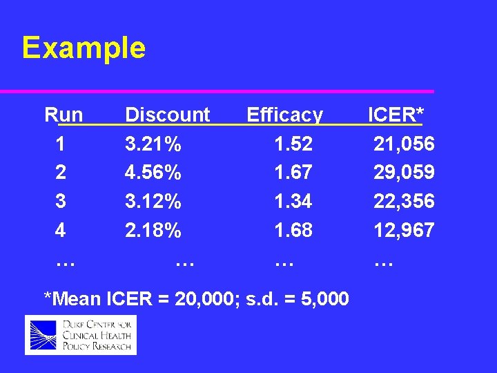
Example Run 1 2 3 4 … Discount 3. 21% 4. 56% 3. 12% 2. 18% … Efficacy 1. 52 1. 67 1. 34 1. 68 … *Mean ICER = 20, 000; s. d. = 5, 000 ICER* 21, 056 29, 059 22, 356 12, 967 …

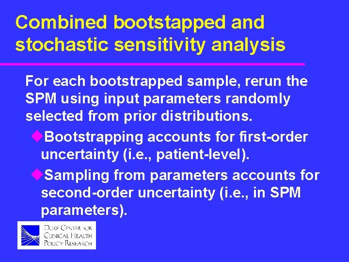
Combined bootstapped and stochastic sensitivity analysis For each bootstrapped sample, rerun the SPM using input parameters randomly selected from prior distributions. u. Bootstrapping accounts for first-order uncertainty (i. e. , patient-level). u. Sampling from parameters accounts for second-order uncertainty (i. e. , in SPM parameters).

Standard of practice The current standard of practice is to use modeling to attach expected values for long -term outcomes to each patient in the trial. One and multi-way sensitivity analyses are performed. Bootstrapping (perhaps combined with stochastic sensitivity analysis) is the state-of-the science, in order to assess the precision associated with the CEA.

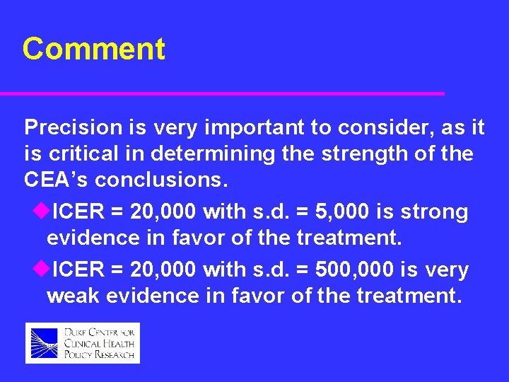
Comment Precision is very important to consider, as it is critical in determining the strength of the CEA’s conclusions. u. ICER = 20, 000 with s. d. = 5, 000 is strong evidence in favor of the treatment. u. ICER = 20, 000 with s. d. = 500, 000 is very weak evidence in favor of the treatment.

SPM structure

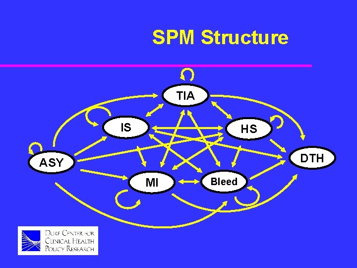
SPM Structure TIA IS HS DTH ASY MI Bleed

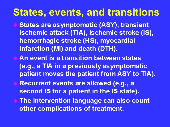
States, events, and transitions u States are asymptomatic (ASY), transient ischemic attack (TIA), ischemic stroke (IS), hemorrhagic stroke (HS), myocardial infarction (MI) and death (DTH). u An event is a transition between states (e. g. , a TIA in a previously asymptomatic patient moves the patient from ASY to TIA). u Recurrent events are allowed (e. g. , a second IS for a patient in the IS state). u The intervention language can also count other complications of treatment.

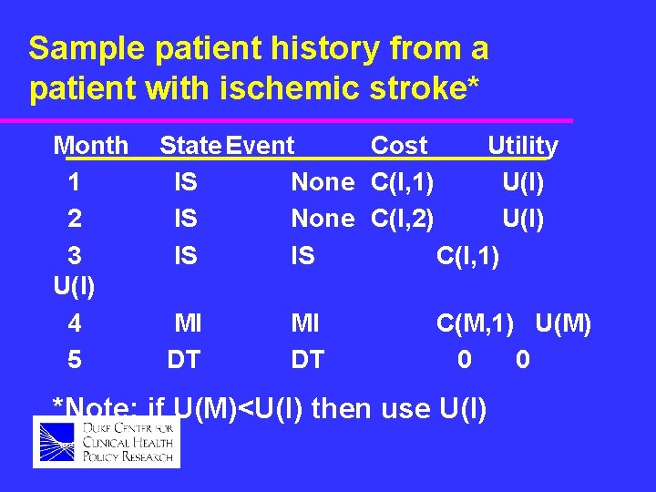
Sample patient history from a patient with ischemic stroke* Month 1 2 3 U(I) 4 5 State Event Cost Utility IS None C(I, 1) U(I) IS None C(I, 2) U(I) IS IS C(I, 1) MI DT C(M, 1) U(M) 0 0 *Note: if U(M)<U(I) then use U(I)

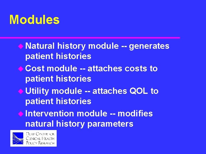
Modules u Natural history module -- generates patient histories u Cost module -- attaches costs to patient histories u Utility module -- attaches QOL to patient histories u Intervention module -- modifies natural history parameters

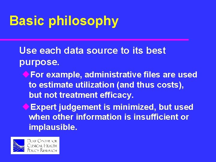
Basic philosophy Use each data source to its best purpose. u. For example, administrative files are used to estimate utilization (and thus costs), but not treatment efficacy. u. Expert judgement is minimized, but used when other information is insufficient or implausible.

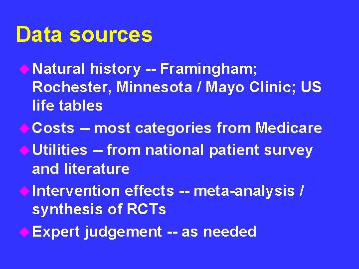
Data sources u Natural history -- Framingham; Rochester, Minnesota / Mayo Clinic; US life tables u Costs -- most categories from Medicare u Utilities -- from national patient survey and literature u Intervention effects -- meta-analysis / synthesis of RCTs u Expert judgement -- as needed

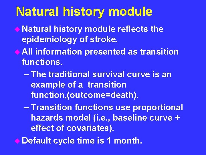
Natural history module u Natural history module reflects the epidemiology of stroke. u All information presented as transition functions. – The traditional survival curve is an example of a transition function, (outcome=death). – Transition functions use proportional hazards model (i. e. , baseline curve + effect of covariates). u Default cycle time is 1 month.

Cost module u The basic idea is that each new event places the patient at “month 0” of a cost curve (reflecting medical costs, over time, after an event such as IS). u Costs can be attached to patient histories either deterministically or stochastically. u Costs are currently in 1996 US dollars.

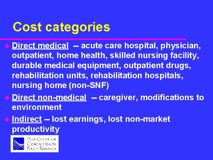
Cost categories u Direct medical -- acute care hospital, physician, outpatient, home health, skilled nursing facility, durable medical equipment, outpatient drugs, rehabilitation units, rehabilitation hospitals, nursing home (non-SNF) u Direct non-medical -- caregiver, modifications to environment u Indirect -- lost earnings, lost non-market productivity

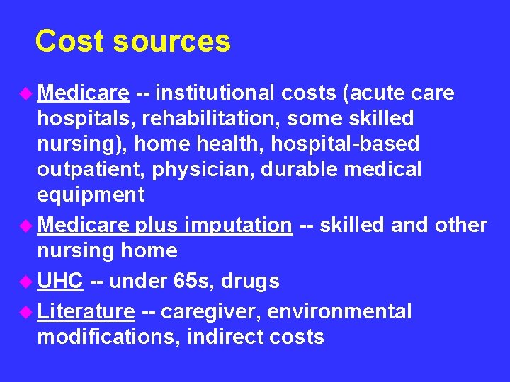
Cost sources u Medicare -- institutional costs (acute care hospitals, rehabilitation, some skilled nursing), home health, hospital-based outpatient, physician, durable medical equipment u Medicare plus imputation -- skilled and other nursing home u UHC -- under 65 s, drugs u Literature -- caregiver, environmental modifications, indirect costs

Utility module u The basic idea is that each event leads to a change (typically, a decrease) in QOL. • Utilities are one measure of QOL u Utilities can be attached to patient histories either deterministically or stochastically.

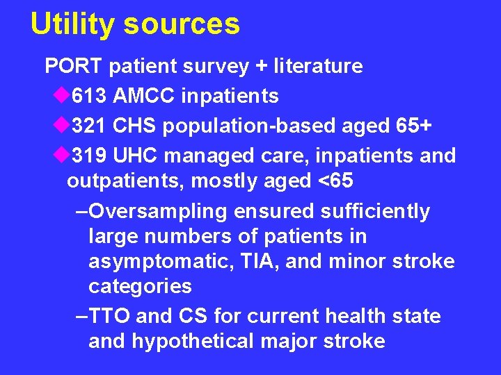
Utility sources PORT patient survey + literature u 613 AMCC inpatients u 321 CHS population-based aged 65+ u 319 UHC managed care, inpatients and outpatients, mostly aged <65 – Oversampling ensured sufficiently large numbers of patients in asymptomatic, TIA, and minor stroke categories – TTO and CS for current health state and hypothetical major stroke

SPM structure -intervention module u Interventions can change natural history, costs, and/or utilities. u Parameters are obtained by metaanalysis / literature synthesis

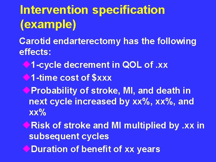
Intervention specification (example) Carotid endarterectomy has the following effects: u 1 -cycle decrement in QOL of. xx u 1 -time cost of $xxx u. Probability of stroke, MI, and death in next cycle increased by xx%, and xx% u. Risk of stroke and MI multiplied by. xx in subsequent cycles u. Duration of benefit of xx years

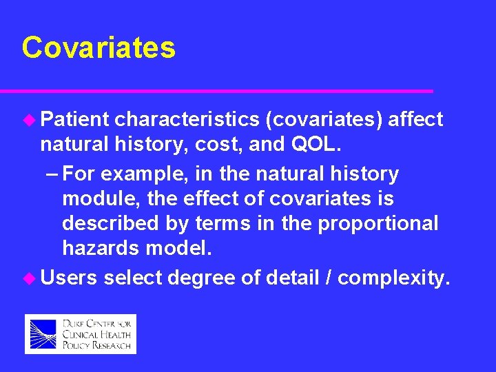
Covariates u Patient characteristics (covariates) affect natural history, cost, and QOL. – For example, in the natural history module, the effect of covariates is described by terms in the proportional hazards model. u Users select degree of detail / complexity.

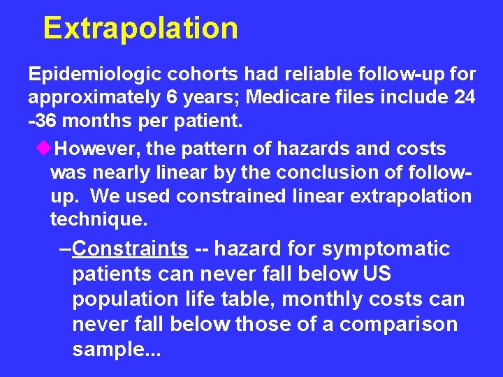
Extrapolation Epidemiologic cohorts had reliable follow-up for approximately 6 years; Medicare files include 24 -36 months per patient. u. However, the pattern of hazards and costs was nearly linear by the conclusion of followup. We used constrained linear extrapolation technique. – Constraints -- hazard for symptomatic patients can never fall below US population life table, monthly costs can never fall below those of a comparison sample. . .

Discounting u Discount rate can be varied. u Default is to discount both life years and costs by 3% risk-less rate.

SPM outputs u Survival u Quality-adjusted survival u Event-free survival u Costs by category u Patient histories